示例4：相场模型

在这个示例中，我们考虑一个二维相场模型：

\[E(\phi) = \int_{\Omega} \left( \frac{\kappa}{2} |\nabla \phi|^2 + \frac{1}{4} (1 - \phi^2)^2 \right) dx\]

Allen-Cahn 方程如下：

\[\dot{\phi} = \kappa \Delta \phi + \phi - \phi^3\]

我们考虑定义域 $\Omega = [0,1]^{2}$ ，并采用周期性边界条件。我们使用有限差分法对其进行离散化，网格划分为 $64 \times 64$。

首先，我们将 saddlescape-1.0 目录的路径添加到系统路径中：

import sys
import os

sys.path.append(os.path.abspath(os.path.join(os.getcwd(), '..', 'saddlescape-1.0')))

接着，我们导入主类：

from saddlescape import Landscape
import numpy as np

# import packages needed

定义能量函数：

from scipy.ndimage import convolve

def gradient_PF(x, opt):
	kappa = opt['kappa']
	n2 = len(x)
	n = int(np.sqrt(n2))
	phi = x.reshape(n, n)
	h = opt['h']

	D2 = np.array([[0, 1, 0],
				   [1, -4, 1],
				   [0, 1, 0]]) / h**2

	conv_term = convolve(phi, D2, mode='wrap')

	F = -(kappa * conv_term + phi - phi**3)

	return F.reshape(n2, 1)

接着，我们定义了具有平移不变性的判断函数。

def SameSaddle(x, y):
	n= 64
	A = x.reshape(n,n)
	B = y.reshape(n,n)
	epsilon = 0.05

	row_indices = np.array([(np.arange(n) - dx) % n for dx in range(n)])
	col_indices = np.array([(np.arange(n) - dy) % n for dy in range(n)])

	row_shifted = np.zeros((n, n, n), dtype=B.dtype)
	for dx in range(n):
		row_shifted[dx] = B[row_indices[dx], :]

	for dx in range(n):
		for dy in range(n):
			shifted_B = row_shifted[dx][:, col_indices[dy]]
			max_diff = np.max(np.abs(A - shifted_B))
			if max_diff <= epsilon:
				return True
	return False

定义系统参数$\kappa=0.02$.

# parameter initialization
x0 = np.array([0 for i in range(N**2)]) # initial point
dt = 1e-3 # time step
k = 5
acceme = 'nesterov'
neschoice = 1
nesres = 200
mom = 0.8
maxiter = 2000 # max iter

MyLandscape = Landscape(MaxIndex=k, AutoDiff=False, Grad=GradFunc, DimerLength=1e-3, 
						HessianDimerLength=1e-3, EigenStepSize=1e-7, InitialPoint=x0, 
						TimeStep=dt, Acceleration=acceme, SearchArea=1e4, SymmetryCheck=False,
						Tolerance=1e-4, MaxIndexGap=3, EigenCombination='min',
						BBStep=True, NesterovChoice=neschoice, NesterovRestart=nesres, 
						Momentum=mom, MaxIter=maxiter, Verbose=True, ReportInterval=10, 
						EigenMaxIter=2, PerturbationNumber=1, EigvecUnified=True,
						SameJudgementMethod=SameSaddle, PerturbationRadius=5.0)
# Instantiation
MyLandscape.Run()
# Calculate

HiSD Solver Configuration:
------------------------------
[HiSD] Current parameters (initialized):
[Config Sync] `Dim` parameter auto-adjusted to 4096 based on `InitialPoint` dimensionality.
Parameter `NumericalGrad` not specified - using default value False.
Parameter `EigenMethod` not specified - using default value lobpcg.
Parameter `ExactHessian` not specified - using default value False.
Parameter `PrecisionTol` not specified - using default value 1e-05.
Parameter 'GradientSystem' not provided. Enabling automatic symmetry detection.


Non-gradient system detected. Activating GHiSD algorithm.
'lobpcg' incompatible with non-gradient systems. Reverting to 'power' method.


Landscape Configuration:
------------------------------
[Landscape] Current parameters (initialized):
Parameter `PerturbationMethod` not specified - using default value uniform.
Parameter `InitialEigenVectors` not specified - using default value None.

Start running:
------------------------------



From initial point search index-5:
------------------------------


Non-degenerate saddle point identified: Morse index =5 (number of negative eigenvalues).


From saddle point (index-5, ID-0) search index-4:
------------------------------


Iteration: 10|| Norm of gradient: 2.626117
Iteration: 20|| Norm of gradient: 2.073056
Iteration: 30|| Norm of gradient: 1.778669
Iteration: 40|| Norm of gradient: 1.685068
Iteration: 50|| Norm of gradient: 1.643202
Iteration: 60|| Norm of gradient: 4.551244
Iteration: 70|| Norm of gradient: 2.191489
Iteration: 80|| Norm of gradient: 1.932887
Iteration: 90|| Norm of gradient: 1.624164
Iteration: 100|| Norm of gradient: 1.375257
Iteration: 110|| Norm of gradient: 1.139303
Iteration: 120|| Norm of gradient: 0.913087
Iteration: 130|| Norm of gradient: 0.756791
Iteration: 140|| Norm of gradient: 0.647716
Iteration: 150|| Norm of gradient: 0.592122
Iteration: 160|| Norm of gradient: 0.578698
Iteration: 170|| Norm of gradient: 0.567598
Iteration: 180|| Norm of gradient: 0.548581
Iteration: 190|| Norm of gradient: 0.516373
Iteration: 200|| Norm of gradient: 0.466288
Iteration: 210|| Norm of gradient: 0.282131
Iteration: 220|| Norm of gradient: 0.269620
Iteration: 230|| Norm of gradient: 0.253248
Iteration: 240|| Norm of gradient: 0.234388
Iteration: 250|| Norm of gradient: 0.213168
Iteration: 260|| Norm of gradient: 0.190388
Iteration: 270|| Norm of gradient: 0.166994
Iteration: 280|| Norm of gradient: 0.143766
Iteration: 290|| Norm of gradient: 0.121361
Iteration: 300|| Norm of gradient: 0.100343
Iteration: 310|| Norm of gradient: 0.081218
Iteration: 320|| Norm of gradient: 0.064524
Iteration: 330|| Norm of gradient: 0.050891
Iteration: 340|| Norm of gradient: 0.040991
Iteration: 350|| Norm of gradient: 0.035177
Iteration: 360|| Norm of gradient: 0.032834
Iteration: 370|| Norm of gradient: 0.032392
Iteration: 380|| Norm of gradient: 0.032298
Iteration: 390|| Norm of gradient: 0.031682
Iteration: 400|| Norm of gradient: 0.030207
Iteration: 410|| Norm of gradient: 0.024279
Iteration: 420|| Norm of gradient: 0.023424
Iteration: 430|| Norm of gradient: 0.022173
Iteration: 440|| Norm of gradient: 0.020657
Iteration: 450|| Norm of gradient: 0.018927
Iteration: 460|| Norm of gradient: 0.017052
Iteration: 470|| Norm of gradient: 0.015098
Iteration: 480|| Norm of gradient: 0.013126
Iteration: 490|| Norm of gradient: 0.011190
Iteration: 500|| Norm of gradient: 0.009342
Iteration: 510|| Norm of gradient: 0.007631
Iteration: 520|| Norm of gradient: 0.006112
Iteration: 530|| Norm of gradient: 0.004849
Iteration: 540|| Norm of gradient: 0.003910
Iteration: 550|| Norm of gradient: 0.003333
Iteration: 560|| Norm of gradient: 0.003077
Iteration: 570|| Norm of gradient: 0.003009
Iteration: 580|| Norm of gradient: 0.002989
Iteration: 590|| Norm of gradient: 0.002935
Iteration: 600|| Norm of gradient: 0.002811
Iteration: 610|| Norm of gradient: 0.002310
Iteration: 620|| Norm of gradient: 0.002230
Iteration: 630|| Norm of gradient: 0.002112
Iteration: 640|| Norm of gradient: 0.001969
Iteration: 650|| Norm of gradient: 0.001805
Iteration: 660|| Norm of gradient: 0.001626
Iteration: 670|| Norm of gradient: 0.001440
Iteration: 680|| Norm of gradient: 0.001251
Iteration: 690|| Norm of gradient: 0.001065
Iteration: 700|| Norm of gradient: 0.000888
Iteration: 710|| Norm of gradient: 0.000724
Iteration: 720|| Norm of gradient: 0.000579
Iteration: 730|| Norm of gradient: 0.000460
Iteration: 740|| Norm of gradient: 0.000371
Iteration: 750|| Norm of gradient: 0.000317
Iteration: 760|| Norm of gradient: 0.000293
Iteration: 770|| Norm of gradient: 0.000286
Iteration: 780|| Norm of gradient: 0.000283
Iteration: 790|| Norm of gradient: 0.000278
Iteration: 800|| Norm of gradient: 0.000266
Iteration: 810|| Norm of gradient: 0.000218
Iteration: 820|| Norm of gradient: 0.000211
Iteration: 830|| Norm of gradient: 0.000200
Iteration: 840|| Norm of gradient: 0.000186
Iteration: 850|| Norm of gradient: 0.000171
Iteration: 860|| Norm of gradient: 0.000154
Iteration: 870|| Norm of gradient: 0.000137
Iteration: 880|| Norm of gradient: 0.000119
Iteration: 890|| Norm of gradient: 0.000101
[WARNING] Degenerate saddle point detected under precision tol=1e-05: Hessian matrix may contain zero eigenvalue(s).
Eigenvalue spectrum: negative=2, zero=2, positive=4092. 

……(完整的结果请参考GitHub仓库中的文件)

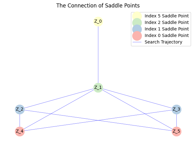
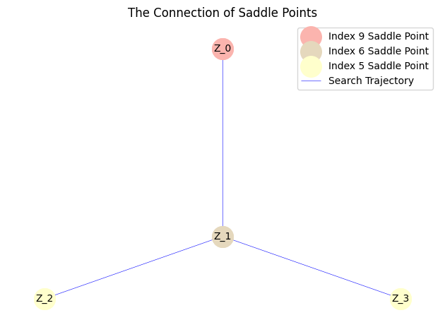
我们可以绘制解景观并保存数据。

MyLandscape.DrawConnection()
MyLandscape.Save('output/Ex_PhaseField','mat')
# Save the data

png

然后，我们可以通过后处理来绘制该函数。

import matplotlib.pyplot as plt
from scipy.interpolate import griddata

def plot_phi_heatmap(phi_vector, N):
    if len(phi_vector) != N * N:
        raise ValueError(f"Input shape must be {N * N}, but got {len(phi_vector)}")
    
    h=1/N

    x = np.linspace(h/2, 1-h/2, N)
    y = np.linspace(h/2, 1-h/2, N)
    X, Y = np.meshgrid(x, y)

    phi = phi_vector.reshape((N, N))

    grid_x, grid_y = np.mgrid[0:1:N*10j, 0:1:N*10j] 
    grid_phi = griddata((X.flatten(), Y.flatten()), phi.flatten(), (grid_x, grid_y), method='cubic')

    # Draw heatmap
    plt.figure(figsize=(8, 6))
    plt.imshow(grid_phi, extent=(0, 1, 0, 1), origin='lower', cmap='viridis',vmin=-1, vmax=1)
    plt.colorbar(label='$\phi$ value')
    plt.title('phase field $\phi$ heatmap')
    plt.xlabel('x')
    plt.ylabel('y')
    plt.show()

for i in range(len(MyLandscape.SaddleList)):
    plot_phi_heatmap(MyLandscape.SaddleList[i][1],N)

png

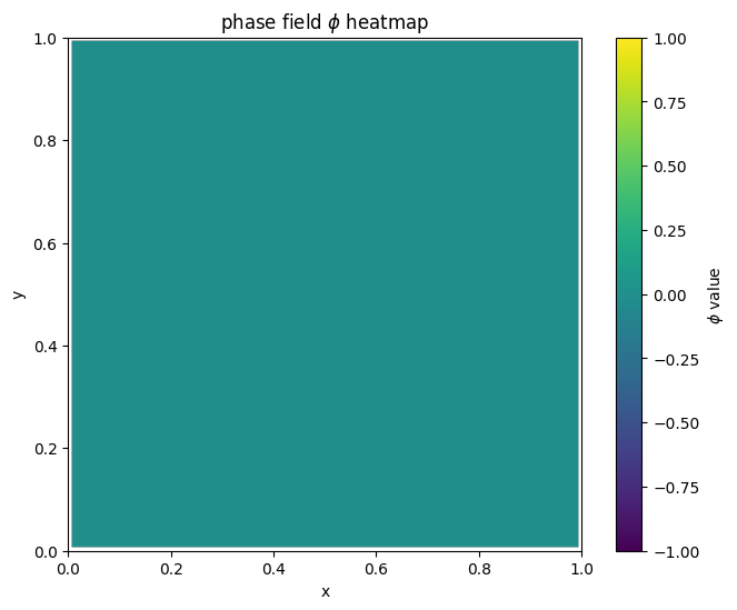
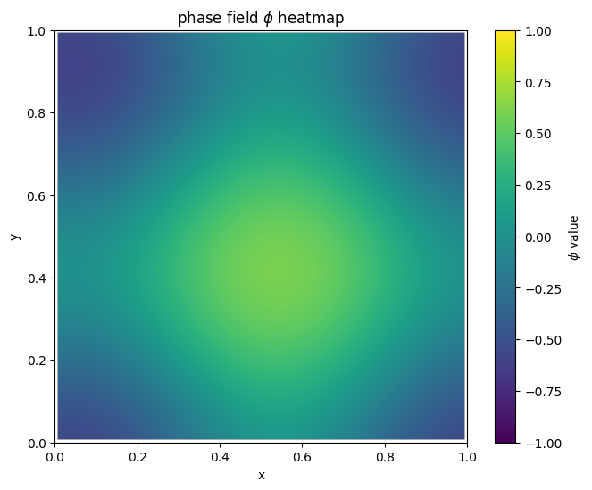
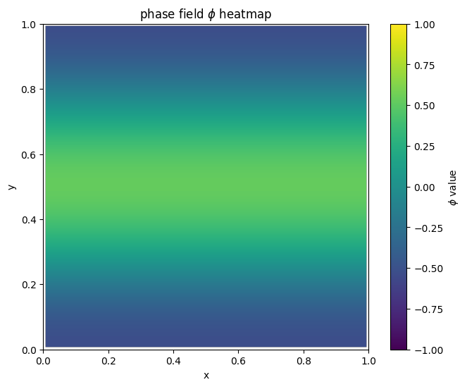
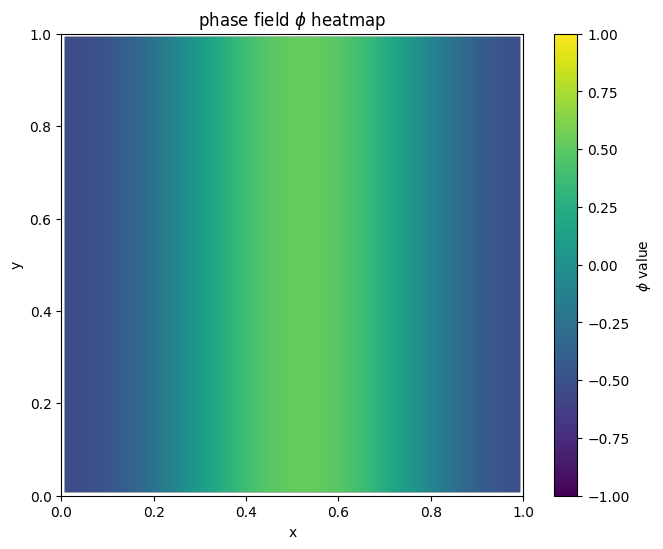
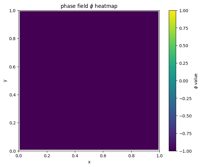
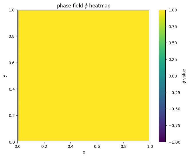
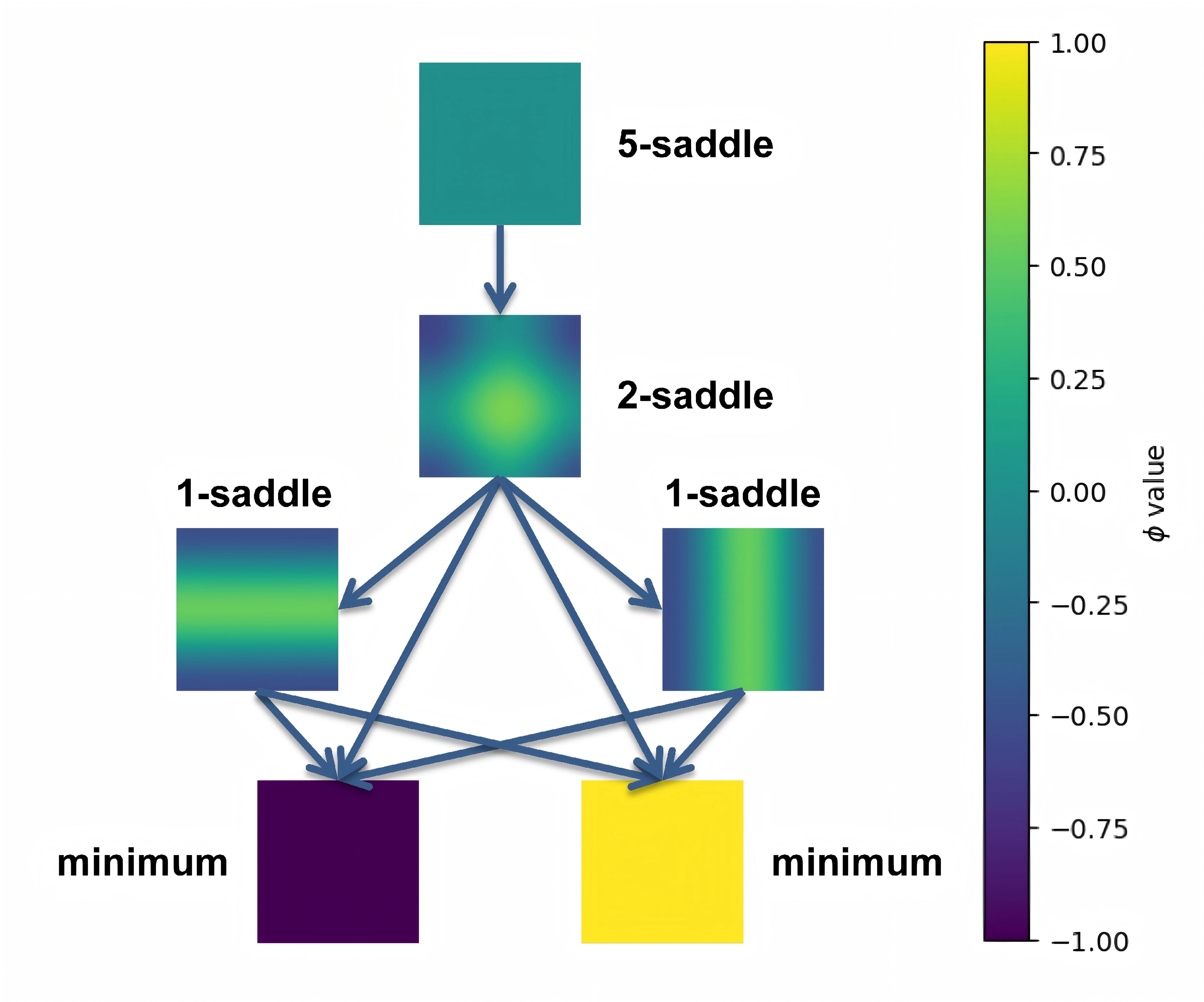
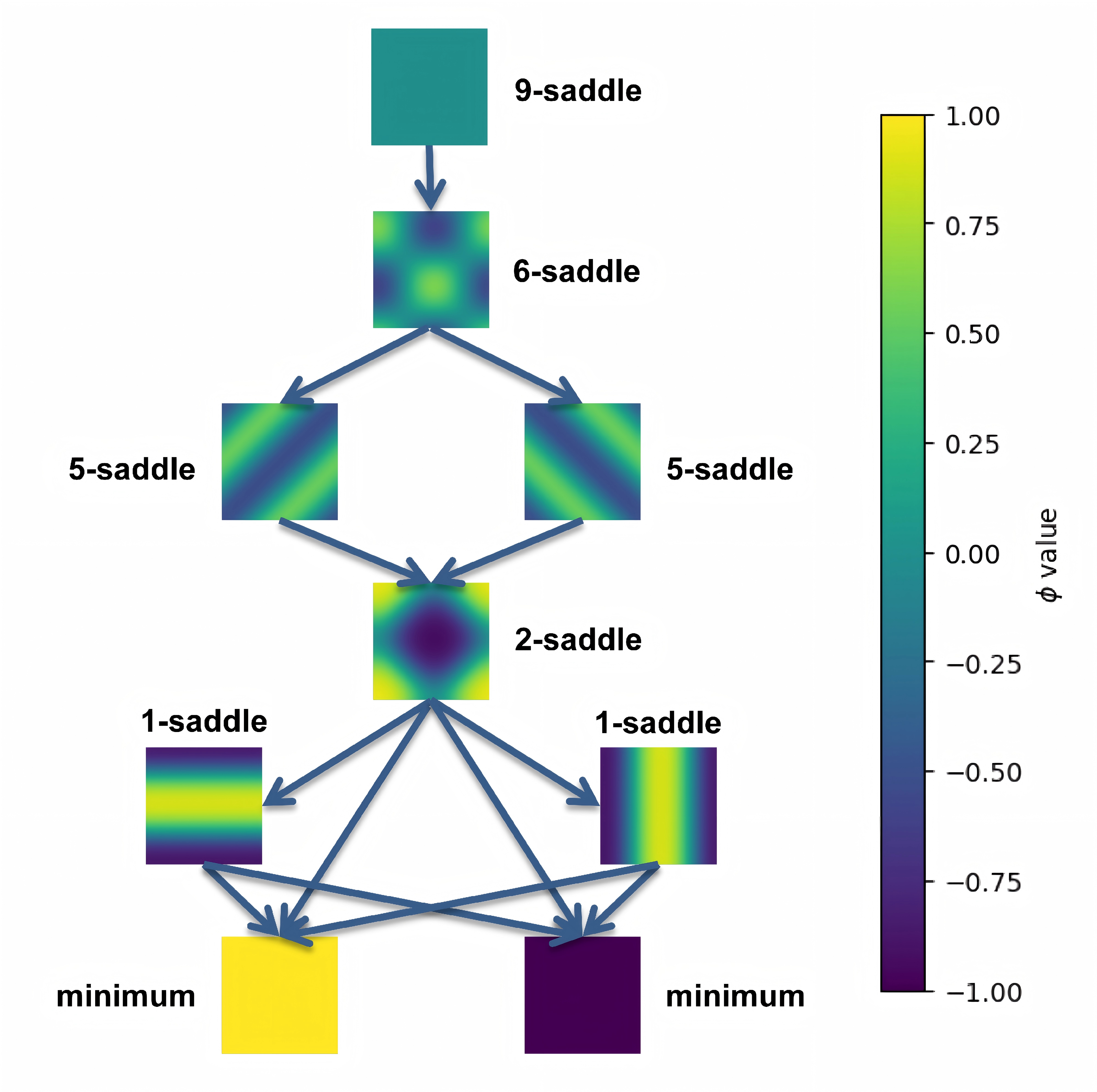
我们把鞍点相场示意图结合解景观联系起来可以得到： png

此外，对于具有更复杂解景观的 $\kappa=0.01$ 系统，我们可以先采用BB步长配合Nesterov加速来快速获取初步的解景观。

png

然而，由于BB步长在梯度较大区域可能变得过大，导致算法发散和搜索不完整，我们随后使用固定小步长重新启动搜索，以构建完整的解景观。这种先加速后精细搜索的两阶段策略有效平衡了计算效率和解的准确性。通过此方法获得的最终解景观如下：

png

(完整的结果请参考GitHub仓库中的文件)

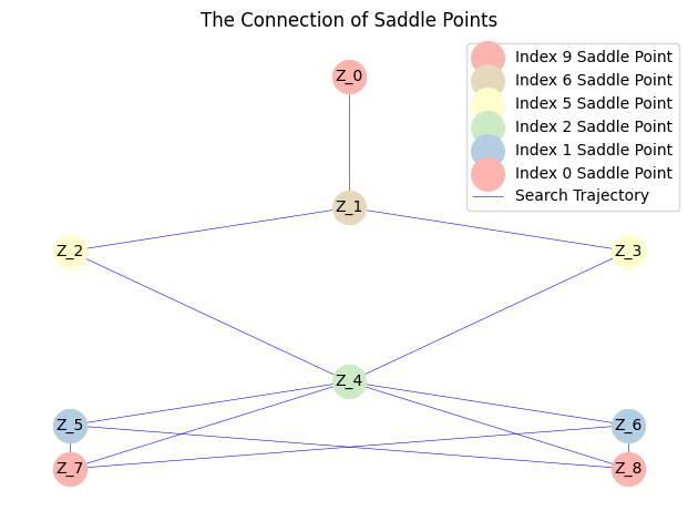
类似上面$\kappa=0.02$的情形我们可以手动绘制如下图形：

png

另外，我们也可以基于快速傅里叶变换(FFT)的归一化互相关来定义判断函数，并获得相同的结果(Ex_4_PhaseField-NewSameSaddle,Ex_4_PhaseField-NewKappa-NewSameSaddle)。

import numpy as np
from numpy.fft import fft2, ifft2

def SameSaddle(x, y):
    """
    Determine if two solutions are equivalent under periodic translation
    using normalized cross-correlation.
    
    Correctly distinguishes A vs shifted(A) (True) from A vs shifted(-A) (False),
    even for self-antisymmetric cases.
    """
    n = 64
    A = x.reshape(n, n)
    B = y.reshape(n, n)

    # 2D Fourier transforms
    fft_A = fft2(A)
    fft_B = fft2(B)
    
    # Cross-correlation spectrum in frequency domain
    cross_corr_spectrum = np.conj(fft_A) * fft_B
    
    # Inverse transform to real space
    real_space_corr = np.real(ifft2(cross_corr_spectrum))
    
    # Find maximum correlation
    max_corr = np.max(real_space_corr)
    
    # Normalization factor (energy of A)
    norm_factor = np.sum(A**2)
    if norm_factor < 1e-7:
        # Zero field case
        return np.sum(B**2) < 1e-7

    # Normalized peak correlation
    normalized_max_corr = max_corr / norm_factor

    # Threshold for equivalence
    if normalized_max_corr > 0.99:
        return True
    
    return False