示例2：Müller-Brown 势能

我们测试由Müller-Brown势函数给出的示例:

\[\begin{aligned} E_{MB}(x,y)=\sum_{i=1}^{4}A_{i}\exp [a_{i}(x-\bar{x}_{i})^{2}+b_{i}(x-\bar{x}_{i})(y-\bar{y}_{i})+c_{i}(y-\bar{y}_{i})^{2}]. \end{aligned}\]

我们将参数设置为：

\[\begin{aligned} A &= [-200,-100,-170,15], \\ a &= [-1,-1,-6.5,0.7], b=[0,0,11,0.6], c=[-10,-10,-6.5,0.7], \\ \bar{x} &= [1,0,-0.5,-1], \bar{y}=[0,0.5,1.5,1]. \end{aligned}\]

首先，我们将 saddlescape-1.0 目录的路径添加到系统路径中：

import sys
import os

sys.path.append(os.path.abspath(os.path.join(os.getcwd(), '..', 'saddlescape-1.0')))

接着，我们导入主类：

from saddlescape import Landscape
import numpy as np

# import packages needed

定义能量函数：

MBP_energyfunc='-200*exp(-1*(x1-1)**2-10*(x2-0)**2)-100*exp(-1*(x1-0)**2-10*(x2-0.5)**2)-170*exp(-6.5*(x1+0.5)**2' \
'+11*(x1+0.5)*(x2-1.5)-6.5*(x2-1.5)**2)+15*exp(0.7*(x1+1)**2+0.6*(x1+1)*(x2-1)+0.7*(x2-1)**2)'

初始化求解器并运行它：

# parameter initialization
x0 = np.array([0.15, 0.25]) # initial point
dt = 4e-4 # time step
k = 1 # the maximum index of saddle point
acceme = 'none' # use the heavy ball to accelerate
maxiter = 5000 # max iter

MyLandscape = Landscape(MaxIndex=k, AutoDiff=True, ExactHessian=True, EnergyFunction=MBP_energyfunc, 
                        InitialPoint=x0, TimeStep=dt, Acceleration=acceme,
                        EigenStepSize=1e-7, MaxIter=maxiter,EigenMethod='euler', Verbose=True, ReportInterval=100)
# Instantiation
MyLandscape.Run()
# Calculate

HiSD Solver Configuration:
------------------------------
[HiSD] Current parameters (initialized):
[Config Sync] `Dim` parameter auto-adjusted to 2 based on `InitialPoint` dimensionality.
Parameter `NumericalGrad` not specified - using default value False.
Parameter `Momentum` not specified - using default value 0.0.
Parameter `BBStep` not specified - using default value False.
Parameter `DimerLength` not specified - using default value 1e-05.
Parameter `Tolerance` not specified - using default value 1e-06.
Parameter `NesterovChoice` not specified - using default value 1.
Parameter `SearchArea` not specified - using default value 1000.0.
Parameter `NesterovRestart` not specified - using default value None.
Parameter `EigenMaxIter` not specified - using default value 10.
Parameter `HessianDimerLength` not specified - using default value 1e-05.
Parameter `PrecisionTol` not specified - using default value 1e-05.
Parameter `EigvecUnified` not specified - using default value False.
Parameter 'GradientSystem' not provided. Enabling automatic symmetry detection.
Parameter 'SymmetryCheck' not provided. Defaulting to True with automatic detection if available.


Gradient system detected. Activating HiSD algorithm.


Landscape Configuration:
------------------------------
[Landscape] Current parameters (initialized):
Parameter `SameJudgementMethod` not specified - using default value <function LandscapeCheckParam.<locals>.<lambda> at 0x0000028FB799E830>.
Parameter `PerturbationMethod` not specified - using default value uniform.
Parameter `PerturbationRadius` not specified - using default value 0.0001.
Parameter `InitialEigenVectors` not specified - using default value None.
Parameter `PerturbationNumber` not specified - using default value 2.
Parameter `SaveTrajectory` not specified - using default value True.
Parameter `MaxIndexGap` not specified - using default value 1.
Parameter `EigenCombination` not specified - using default value all.

Start running:
------------------------------



From initial point search index-1:
------------------------------


Non-degenerate saddle point identified: Morse index =1 (number of negative eigenvalues).


From saddle point (index-1, ID-0) search index-0:
------------------------------


Iteration: 100|| Norm of gradient: 0.070041
Iteration: 200|| Norm of gradient: 0.000007
Non-degenerate saddle point identified: Morse index =0 (number of negative eigenvalues).


From saddle point (index-1, ID-0) search index-0:
------------------------------


Iteration: 100|| Norm of gradient: 0.000010
Non-degenerate saddle point identified: Morse index =0 (number of negative eigenvalues).


From saddle point (index-1, ID-0) search index-0:
------------------------------


Iteration: 100|| Norm of gradient: 0.000010
Non-degenerate saddle point identified: Morse index =0 (number of negative eigenvalues).


From saddle point (index-1, ID-0) search index-0:
------------------------------


Iteration: 100|| Norm of gradient: 0.070041
Iteration: 200|| Norm of gradient: 0.000007
Non-degenerate saddle point identified: Morse index =0 (number of negative eigenvalues).

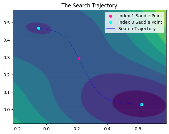
我们可以绘制搜索轨迹。

MyLandscape.DrawTrajectory(ContourGridNum=100, ContourGridOut=25, DetailedTraj=True)
# Draw the search path. But because of the large dimension, we cannot draw the picture.

我们也可以绘制解景观。

MyLandscape.DrawConnection()

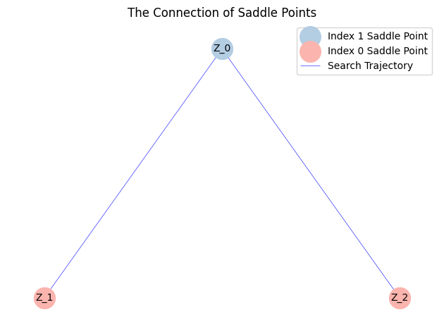
然而，Müller-Brown势描述了一个具有多峰分布的典型系统。因此，上面展示的解景观并不完整。于是，我们从局部最小值重新开始搜索：

MyLandscape.RestartFromSaddle(1,-np.array([[-0.01],[0]]),1)
# Calculate

From initial point search index-1:
------------------------------


Iteration: 100|| Norm of gradient: 3.005940
Iteration: 200|| Norm of gradient: 0.692884
Iteration: 300|| Norm of gradient: 0.000017
Non-degenerate saddle point identified: Morse index =1 (number of negative eigenvalues).


From saddle point (index-1, ID-3) search index-0:
------------------------------


Iteration: 100|| Norm of gradient: 0.002417
Non-degenerate saddle point identified: Morse index =0 (number of negative eigenvalues).


From saddle point (index-1, ID-3) search index-0:
------------------------------


Iteration: 100|| Norm of gradient: 0.343433
Iteration: 200|| Norm of gradient: 0.000033
Non-degenerate saddle point identified: Morse index =0 (number of negative eigenvalues).


From saddle point (index-1, ID-3) search index-0:
------------------------------


Iteration: 100|| Norm of gradient: 0.343433
Iteration: 200|| Norm of gradient: 0.000033
Non-degenerate saddle point identified: Morse index =0 (number of negative eigenvalues).


From saddle point (index-1, ID-3) search index-0:
------------------------------


Iteration: 100|| Norm of gradient: 0.002417
Non-degenerate saddle point identified: Morse index =0 (number of negative eigenvalues).

MyLandscape.DrawTrajectory(ContourGridNum=100, ContourGridOut=25, DetailedTraj=True)
# Draw the search path. But because of the large dimension, we cannot draw the picture.

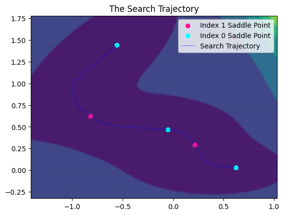
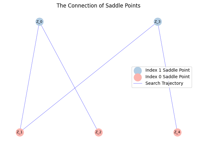
从输出结果中，我们可以得到一个完整的解景观。

MyLandscape.DrawConnection()
MyLandscape.Save('output/Ex_MBP','pickle')
# Save the data