Example 4 : Phase Field
In this example, we consider a 2D phase field model:
\[E(\phi) = \int_{\Omega} \left( \frac{\kappa}{2} |\nabla \phi|^2 + \frac{1}{4} (1 - \phi^2)^2 \right) dx\]The Allen-Cahn equation is:
\[\dot{\phi} = \kappa \Delta \phi + \phi - \phi^3\]We consider $\Omega = [0,1]^{2}$ with periodic boundary condition. We discrete it using finite difference scheme of mesh grids $64 \times 64$.
First, we add the path of the saddlescape-1.0 directory to the system path.
import sys
import os

sys.path.append(os.path.abspath(os.path.join(os.getcwd(), '..', 'saddlescape-1.0')))
Then, we import the main class.
from saddlescape import Landscape
import numpy as np

# import packages needed
We define the vector field by 2-D convolution.
from scipy.ndimage import convolve

def gradient_PF(x, opt):
	kappa = opt['kappa']
	n2 = len(x)
	n = int(np.sqrt(n2))
	phi = x.reshape(n, n)
	h = opt['h']

	D2 = np.array([[0, 1, 0],
				   [1, -4, 1],
				   [0, 1, 0]]) / h**2

	conv_term = convolve(phi, D2, mode='wrap')

	F = -(kappa * conv_term + phi - phi**3)

	return F.reshape(n2, 1)
Then, we define the judgement function with translational invariance.
def SameSaddle(x, y):
	n= 64
	A = x.reshape(n,n)
	B = y.reshape(n,n)
	epsilon = 0.05

	row_indices = np.array([(np.arange(n) - dx) % n for dx in range(n)])
	col_indices = np.array([(np.arange(n) - dy) % n for dy in range(n)])

	row_shifted = np.zeros((n, n, n), dtype=B.dtype)
	for dx in range(n):
		row_shifted[dx] = B[row_indices[dx], :]

	for dx in range(n):
		for dy in range(n):
			shifted_B = row_shifted[dx][:, col_indices[dy]]
			max_diff = np.max(np.abs(A - shifted_B))
			if max_diff <= epsilon:
				return True
	return False
Define the system with $\kappa=0.02$.
N = 64
opt = {
	'kappa': 0.02,
	'N': N,
	'h': 1/N,
}

GradFunc = lambda x: gradient_PF(x, opt)
We initialize the solver and run it.
# parameter initialization
x0 = np.array([0 for i in range(N**2)]) # initial point
dt = 1e-3 # time step
k = 5
acceme = 'nesterov'
neschoice = 1
nesres = 200
mom = 0.8
maxiter = 2000 # max iter
MyLandscape = Landscape(MaxIndex=k, AutoDiff=False, Grad=GradFunc, DimerLength=1e-3,
						HessianDimerLength=1e-3, EigenStepSize=1e-7, InitialPoint=x0,
						TimeStep=dt, Acceleration=acceme, SearchArea=1e4, SymmetryCheck=False,
						Tolerance=1e-4, MaxIndexGap=3, EigenCombination='min',
						BBStep=True, NesterovChoice=neschoice, NesterovRestart=nesres,
						Momentum=mom, MaxIter=maxiter, Verbose=True, ReportInterval=10,
						EigenMaxIter=2, PerturbationNumber=1, EigvecUnified=True,
						SameJudgementMethod=SameSaddle, PerturbationRadius=5.0)
# Instantiation
MyLandscape.Run()
# Calculate
HiSD Solver Configuration:
------------------------------
[HiSD] Current parameters (initialized):
[Config Sync] `Dim` parameter auto-adjusted to 4096 based on `InitialPoint` dimensionality.
Parameter `NumericalGrad` not specified - using default value False.
Parameter `EigenMethod` not specified - using default value lobpcg.
Parameter `ExactHessian` not specified - using default value False.
Parameter `PrecisionTol` not specified - using default value 1e-05.
Parameter 'GradientSystem' not provided. Enabling automatic symmetry detection.


Non-gradient system detected. Activating GHiSD algorithm.
'lobpcg' incompatible with non-gradient systems. Reverting to 'power' method.


Landscape Configuration:
------------------------------
[Landscape] Current parameters (initialized):
Parameter `PerturbationMethod` not specified - using default value uniform.
Parameter `InitialEigenVectors` not specified - using default value None.

Start running:
------------------------------


From initial point search index-5:
------------------------------


Non-degenerate saddle point identified: Morse index =5 (number of negative eigenvalues).


From saddle point (index-5, ID-0) search index-4:
------------------------------


Iteration: 10|| Norm of gradient: 2.626117
Iteration: 20|| Norm of gradient: 2.073056
Iteration: 30|| Norm of gradient: 1.778669
Iteration: 40|| Norm of gradient: 1.685068
Iteration: 50|| Norm of gradient: 1.643202
Iteration: 60|| Norm of gradient: 4.551244
Iteration: 70|| Norm of gradient: 2.191489
Iteration: 80|| Norm of gradient: 1.932887
Iteration: 90|| Norm of gradient: 1.624164
Iteration: 100|| Norm of gradient: 1.375257
Iteration: 110|| Norm of gradient: 1.139303
Iteration: 120|| Norm of gradient: 0.913087
Iteration: 130|| Norm of gradient: 0.756791
Iteration: 140|| Norm of gradient: 0.647716
Iteration: 150|| Norm of gradient: 0.592122
Iteration: 160|| Norm of gradient: 0.578698
Iteration: 170|| Norm of gradient: 0.567598
Iteration: 180|| Norm of gradient: 0.548581
Iteration: 190|| Norm of gradient: 0.516373
Iteration: 200|| Norm of gradient: 0.466288
Iteration: 210|| Norm of gradient: 0.282131
Iteration: 220|| Norm of gradient: 0.269620
Iteration: 230|| Norm of gradient: 0.253248
Iteration: 240|| Norm of gradient: 0.234388
Iteration: 250|| Norm of gradient: 0.213168
Iteration: 260|| Norm of gradient: 0.190388
Iteration: 270|| Norm of gradient: 0.166994
Iteration: 280|| Norm of gradient: 0.143766
Iteration: 290|| Norm of gradient: 0.121361
Iteration: 300|| Norm of gradient: 0.100343
Iteration: 310|| Norm of gradient: 0.081218
Iteration: 320|| Norm of gradient: 0.064524
Iteration: 330|| Norm of gradient: 0.050891
Iteration: 340|| Norm of gradient: 0.040991
Iteration: 350|| Norm of gradient: 0.035177
Iteration: 360|| Norm of gradient: 0.032834
Iteration: 370|| Norm of gradient: 0.032392
Iteration: 380|| Norm of gradient: 0.032298
Iteration: 390|| Norm of gradient: 0.031682
Iteration: 400|| Norm of gradient: 0.030207
Iteration: 410|| Norm of gradient: 0.024279
Iteration: 420|| Norm of gradient: 0.023424
Iteration: 430|| Norm of gradient: 0.022173
Iteration: 440|| Norm of gradient: 0.020657
Iteration: 450|| Norm of gradient: 0.018927
Iteration: 460|| Norm of gradient: 0.017052
Iteration: 470|| Norm of gradient: 0.015098
Iteration: 480|| Norm of gradient: 0.013126
Iteration: 490|| Norm of gradient: 0.011190
Iteration: 500|| Norm of gradient: 0.009342
Iteration: 510|| Norm of gradient: 0.007631
Iteration: 520|| Norm of gradient: 0.006112
Iteration: 530|| Norm of gradient: 0.004849
Iteration: 540|| Norm of gradient: 0.003910
Iteration: 550|| Norm of gradient: 0.003333
Iteration: 560|| Norm of gradient: 0.003077
Iteration: 570|| Norm of gradient: 0.003009
Iteration: 580|| Norm of gradient: 0.002989
Iteration: 590|| Norm of gradient: 0.002935
Iteration: 600|| Norm of gradient: 0.002811
Iteration: 610|| Norm of gradient: 0.002310
Iteration: 620|| Norm of gradient: 0.002230
Iteration: 630|| Norm of gradient: 0.002112
Iteration: 640|| Norm of gradient: 0.001969
Iteration: 650|| Norm of gradient: 0.001805
Iteration: 660|| Norm of gradient: 0.001626
Iteration: 670|| Norm of gradient: 0.001440
Iteration: 680|| Norm of gradient: 0.001251
Iteration: 690|| Norm of gradient: 0.001065
Iteration: 700|| Norm of gradient: 0.000888
Iteration: 710|| Norm of gradient: 0.000724
Iteration: 720|| Norm of gradient: 0.000579
Iteration: 730|| Norm of gradient: 0.000460
Iteration: 740|| Norm of gradient: 0.000371
Iteration: 750|| Norm of gradient: 0.000317
Iteration: 760|| Norm of gradient: 0.000293
Iteration: 770|| Norm of gradient: 0.000286
Iteration: 780|| Norm of gradient: 0.000283
Iteration: 790|| Norm of gradient: 0.000278
Iteration: 800|| Norm of gradient: 0.000266
Iteration: 810|| Norm of gradient: 0.000218
Iteration: 820|| Norm of gradient: 0.000211
Iteration: 830|| Norm of gradient: 0.000200
Iteration: 840|| Norm of gradient: 0.000186
Iteration: 850|| Norm of gradient: 0.000171
Iteration: 860|| Norm of gradient: 0.000154
Iteration: 870|| Norm of gradient: 0.000137
Iteration: 880|| Norm of gradient: 0.000119
Iteration: 890|| Norm of gradient: 0.000101
[WARNING] Degenerate saddle point detected under precision tol=1e-05: Hessian matrix may contain zero eigenvalue(s).
Eigenvalue spectrum: negative=2, zero=2, positive=4092.
……(For the complete results, please refer to the file in the GitHub repository)
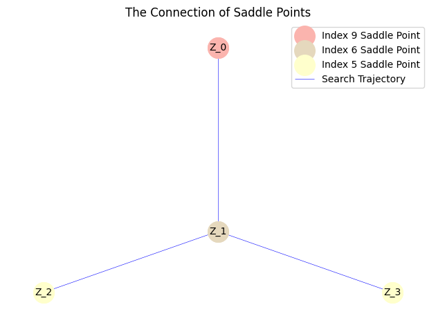
We can draw the solution landscape and save the data.
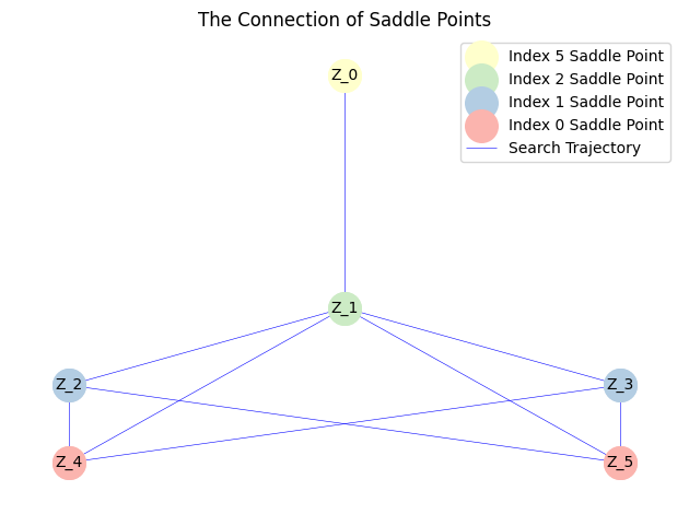
MyLandscape.DrawConnection()
MyLandscape.Save('output/Ex_PhaseField','mat')
# Save the data
Then, we can draw the function by post-processing.
import matplotlib.pyplot as plt
from scipy.interpolate import griddata

def plot_phi_heatmap(phi_vector, N):
	if len(phi_vector) != N * N:
		raise ValueError(f"Input shape must be {N * N}, but got {len(phi_vector)}")

	h=1/N

	x = np.linspace(h/2, 1-h/2, N)
	y = np.linspace(h/2, 1-h/2, N)
	X, Y = np.meshgrid(x, y)

	phi = phi_vector.reshape((N, N))

	grid_x, grid_y = np.mgrid[0:1:N*10j, 0:1:N*10j]
	grid_phi = griddata((X.flatten(), Y.flatten()), phi.flatten(), (grid_x, grid_y), method='cubic')

	# Draw heatmap
	plt.figure(figsize=(8, 6))
	plt.imshow(grid_phi, extent=(0, 1, 0, 1), origin='lower', cmap='viridis',vmin=-1, vmax=1)
	plt.colorbar(label='$\phi$ value')
	plt.title('phase field $\phi$ heatmap')
	plt.xlabel('x')
	plt.ylabel('y')
	plt.show()
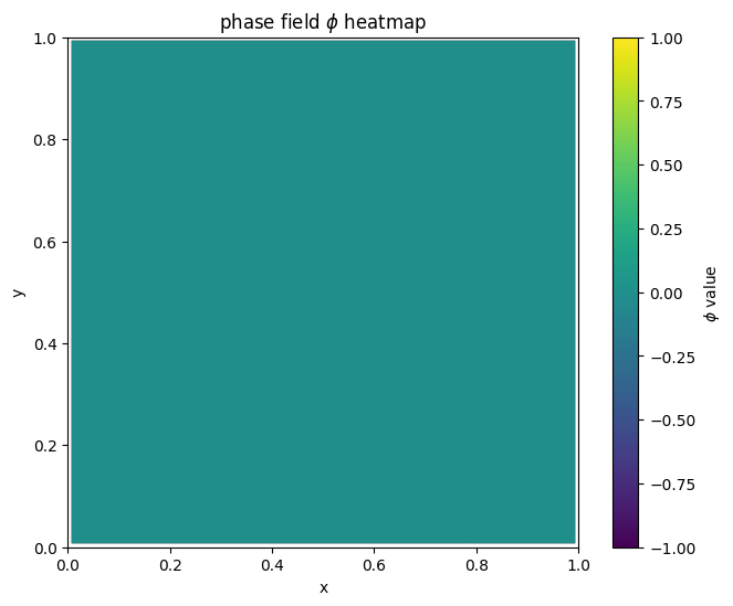
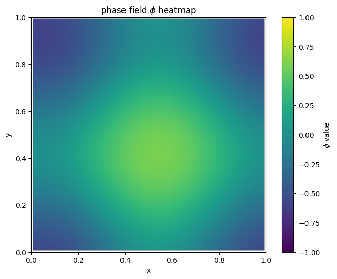
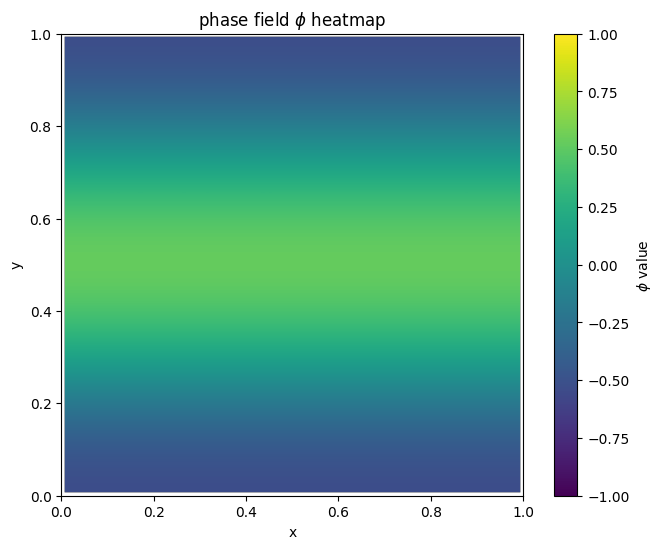
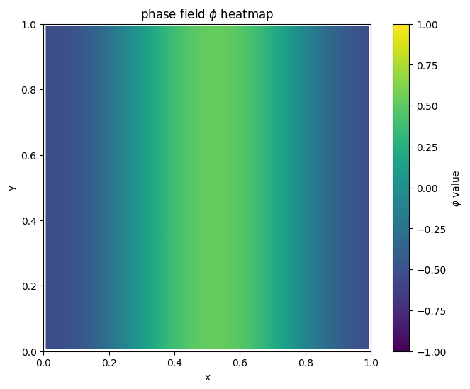
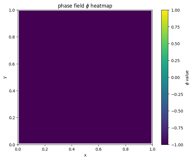
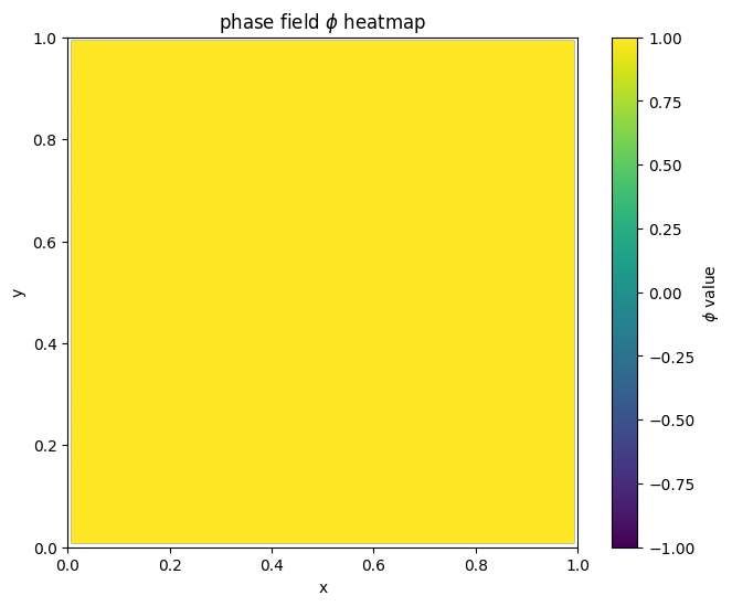
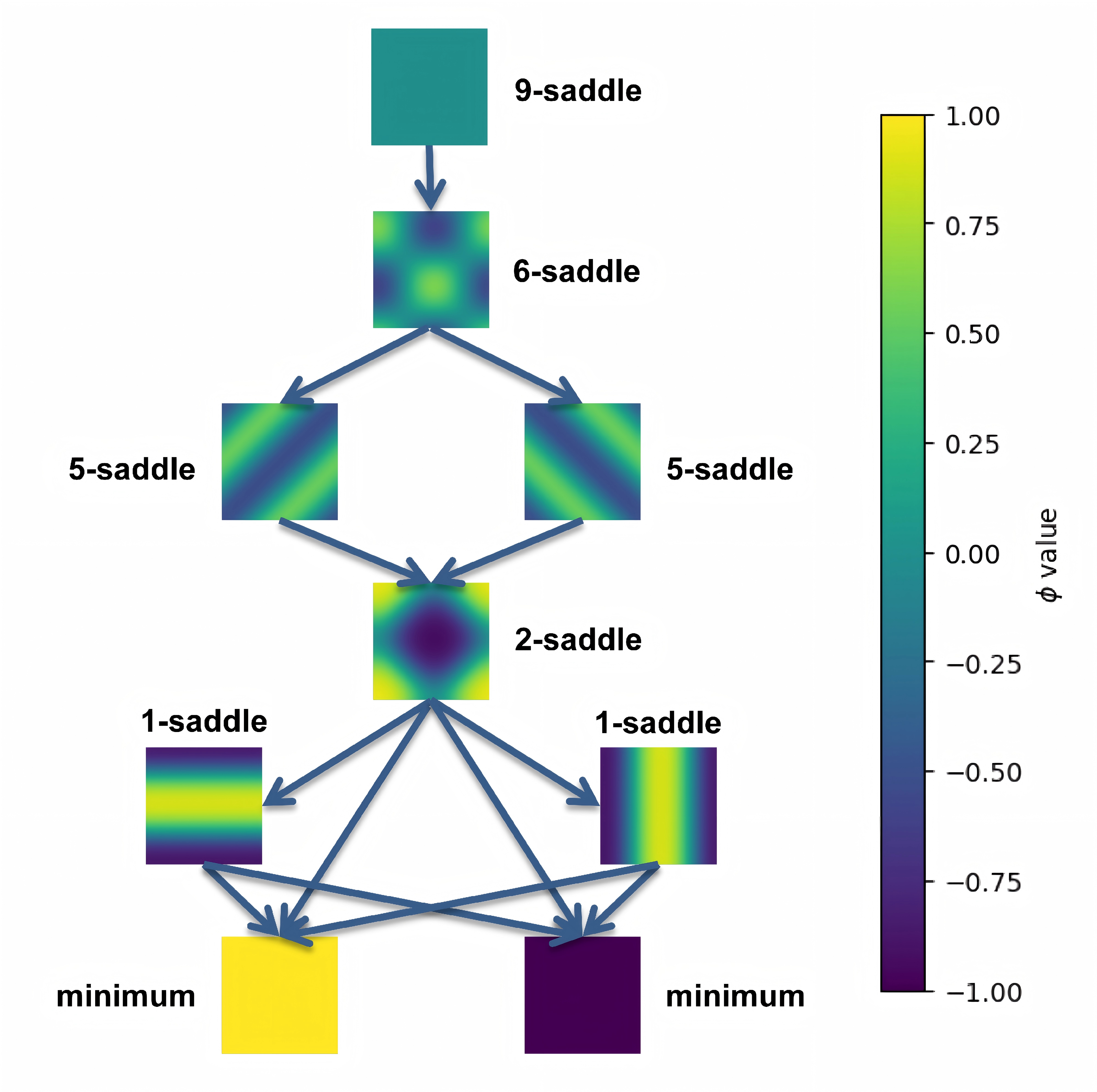
for i in range(len(MyLandscape.SaddleList)):
	plot_phi_heatmap(MyLandscape.SaddleList[i][1],N)
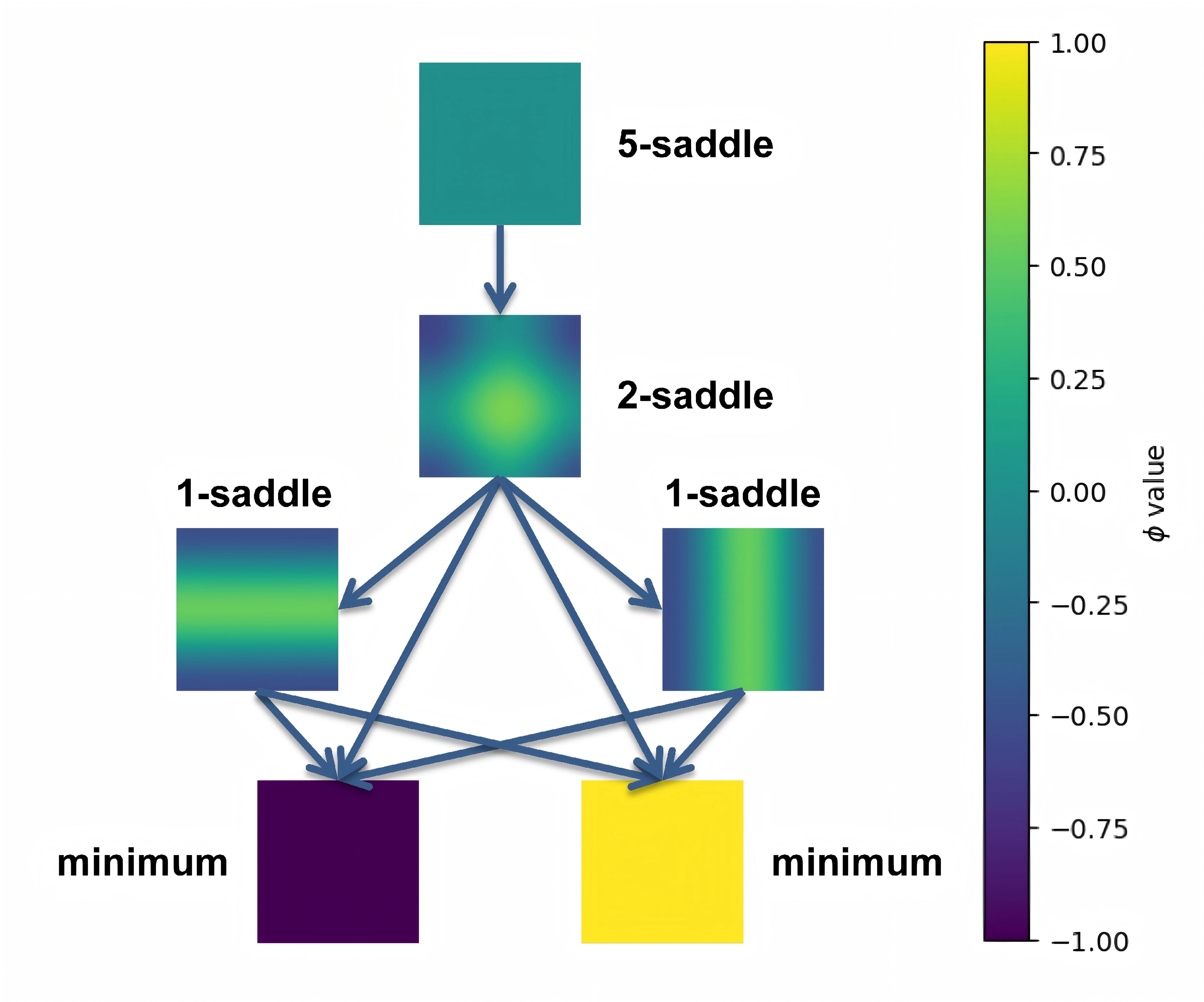
By linking the saddle-point phase field schematic diagram with the solution landscape, we can establish the connection between them:
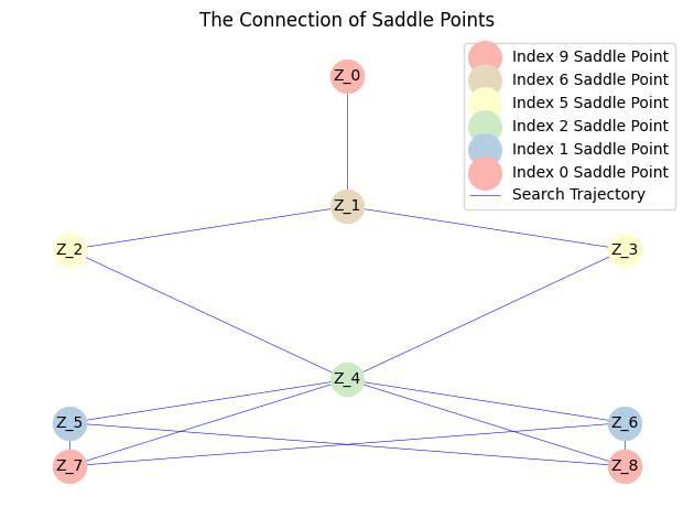
Moreover, for a system with $\kappa=0.01$ that possesses a more complex solution landscape, we can initially employ the fast BB step size combined with Nesterov acceleration to obtain an approximate solution landscape.
However, since the BB step size might become excessively large in regions with steep gradients, potentially leading to algorithm divergence and incomplete exploration, we subsequently restart the search using a fixed small step size to construct the complete solution landscape. This two-stage strategy of accelerated search followed by refined exploration effectively balances computational efficiency and solution accuracy. The final solution landscape obtained through this approach is presented as follows:
(For the complete results, please refer to the file in the GitHub repository)
Similarly to the case of $\kappa=0.02$ above, we can manually draw the following figure:
Besides, we can also define the judgement function with normalized cross-correlation based on Fast Fourier Transform(FFT) and will get the same results(Ex_4_PhaseField-NewSameSaddle,Ex_4_PhaseField-NewKappa-NewSameSaddle).
import numpy as np
from numpy.fft import fft2, ifft2

def SameSaddle(x, y):
    """
    Determine if two solutions are equivalent under periodic translation
    using normalized cross-correlation.

    Correctly distinguishes A vs shifted(A) (True) from A vs shifted(-A) (False),
    even for self-antisymmetric cases.
    """
    n = 64
    A = x.reshape(n, n)
    B = y.reshape(n, n)

    # 2D Fourier transforms
    fft_A = fft2(A)
    fft_B = fft2(B)

    # Cross-correlation spectrum in frequency domain
    cross_corr_spectrum = np.conj(fft_A) * fft_B

    # Inverse transform to real space
    real_space_corr = np.real(ifft2(cross_corr_spectrum))

    # Find maximum correlation
    max_corr = np.max(real_space_corr)

    # Normalization factor (energy of A)
    norm_factor = np.sum(A**2)
    if norm_factor < 1e-7:
        # Zero field case
        return np.sum(B**2) < 1e-7

    # Normalized peak correlation
    normalized_max_corr = max_corr / norm_factor

    # Threshold for equivalence
    if normalized_max_corr > 0.99:
        return True

    return False