Example 2 : Müller-Brown Potential

We test the Müller-Brown potential given by

\[\begin{aligned} E_{MB}(x,y)=\sum_{i=1}^{4}A_{i}\exp [a_{i}(x-\bar{x}_{i})^{2}+b_{i}(x-\bar{x}_{i})(y-\bar{y}_{i})+c_{i}(y-\bar{y}_{i})^{2}]. \end{aligned}\]

We set the parameters as

\[\begin{aligned} A &= [-200,-100,-170,15], \\ a &= [-1,-1,-6.5,0.7], b=[0,0,11,0.6], c=[-10,-10,-6.5,0.7], \\ \bar{x} &= [1,0,-0.5,-1], \bar{y}=[0,0.5,1.5,1]. \end{aligned}\]

First, we add the path of the saddlescape-1.0 directory to the system path.

import sys
import os

sys.path.append(os.path.abspath(os.path.join(os.getcwd(), '..', 'saddlescape-1.0')))

Then, we import the main class.

from saddlescape import Landscape
import numpy as np

# import packages needed

We define the energy function.

MBP_energyfunc='-200*exp(-1*(x1-1)**2-10*(x2-0)**2)-100*exp(-1*(x1-0)**2-10*(x2-0.5)**2)-170*exp(-6.5*(x1+0.5)**2' \
'+11*(x1+0.5)*(x2-1.5)-6.5*(x2-1.5)**2)+15*exp(0.7*(x1+1)**2+0.6*(x1+1)*(x2-1)+0.7*(x2-1)**2)'

We initialize the solver and run it.

# parameter initialization
x0 = np.array([0.15, 0.25]) # initial point
dt = 4e-4 # time step
k = 1 # the maximum index of saddle point
acceme = 'none' # use the heavy ball to accelerate
maxiter = 5000 # max iter

MyLandscape = Landscape(MaxIndex=k, AutoDiff=True, ExactHessian=True, EnergyFunction=MBP_energyfunc, 
                        InitialPoint=x0, TimeStep=dt, Acceleration=acceme,
                        EigenStepSize=1e-7, MaxIter=maxiter,EigenMethod='euler', Verbose=True, ReportInterval=100)
# Instantiation
MyLandscape.Run()
# Calculate

HiSD Solver Configuration:
------------------------------
[HiSD] Current parameters (initialized):
[Config Sync] `Dim` parameter auto-adjusted to 2 based on `InitialPoint` dimensionality.
Parameter `NumericalGrad` not specified - using default value False.
Parameter `Momentum` not specified - using default value 0.0.
Parameter `BBStep` not specified - using default value False.
Parameter `DimerLength` not specified - using default value 1e-05.
Parameter `Tolerance` not specified - using default value 1e-06.
Parameter `NesterovChoice` not specified - using default value 1.
Parameter `SearchArea` not specified - using default value 1000.0.
Parameter `NesterovRestart` not specified - using default value None.
Parameter `EigenMaxIter` not specified - using default value 10.
Parameter `HessianDimerLength` not specified - using default value 1e-05.
Parameter `PrecisionTol` not specified - using default value 1e-05.
Parameter `EigvecUnified` not specified - using default value False.
Parameter 'GradientSystem' not provided. Enabling automatic symmetry detection.
Parameter 'SymmetryCheck' not provided. Defaulting to True with automatic detection if available.


Gradient system detected. Activating HiSD algorithm.


Landscape Configuration:
------------------------------
[Landscape] Current parameters (initialized):
Parameter `SameJudgementMethod` not specified - using default value <function LandscapeCheckParam.<locals>.<lambda> at 0x0000028FB799E830>.
Parameter `PerturbationMethod` not specified - using default value uniform.
Parameter `PerturbationRadius` not specified - using default value 0.0001.
Parameter `InitialEigenVectors` not specified - using default value None.
Parameter `PerturbationNumber` not specified - using default value 2.
Parameter `SaveTrajectory` not specified - using default value True.
Parameter `MaxIndexGap` not specified - using default value 1.
Parameter `EigenCombination` not specified - using default value all.

Start running:
------------------------------



From initial point search index-1:
------------------------------


Non-degenerate saddle point identified: Morse index =1 (number of negative eigenvalues).


From saddle point (index-1, ID-0) search index-0:
------------------------------


Iteration: 100|| Norm of gradient: 0.070041
Iteration: 200|| Norm of gradient: 0.000007
Non-degenerate saddle point identified: Morse index =0 (number of negative eigenvalues).


From saddle point (index-1, ID-0) search index-0:
------------------------------


Iteration: 100|| Norm of gradient: 0.000010
Non-degenerate saddle point identified: Morse index =0 (number of negative eigenvalues).


From saddle point (index-1, ID-0) search index-0:
------------------------------


Iteration: 100|| Norm of gradient: 0.000010
Non-degenerate saddle point identified: Morse index =0 (number of negative eigenvalues).


From saddle point (index-1, ID-0) search index-0:
------------------------------


Iteration: 100|| Norm of gradient: 0.070041
Iteration: 200|| Norm of gradient: 0.000007
Non-degenerate saddle point identified: Morse index =0 (number of negative eigenvalues).

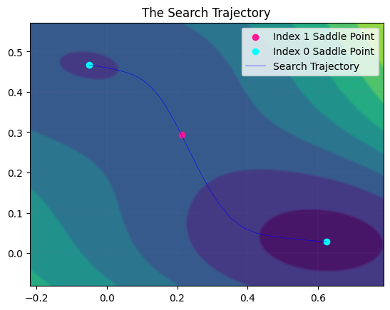
We draw the search trajectory.

MyLandscape.DrawTrajectory(ContourGridNum=100, ContourGridOut=25, DetailedTraj=True)
# Draw the search path. But because of the large dimension, we cannot draw the picture.

We can also draw the solution landscape.

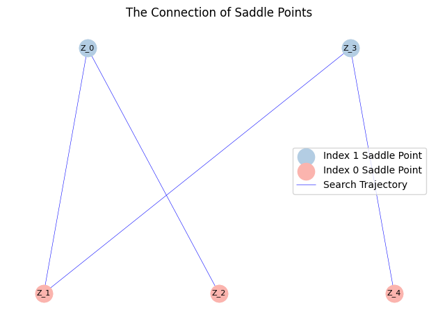
MyLandscape.DrawConnection()

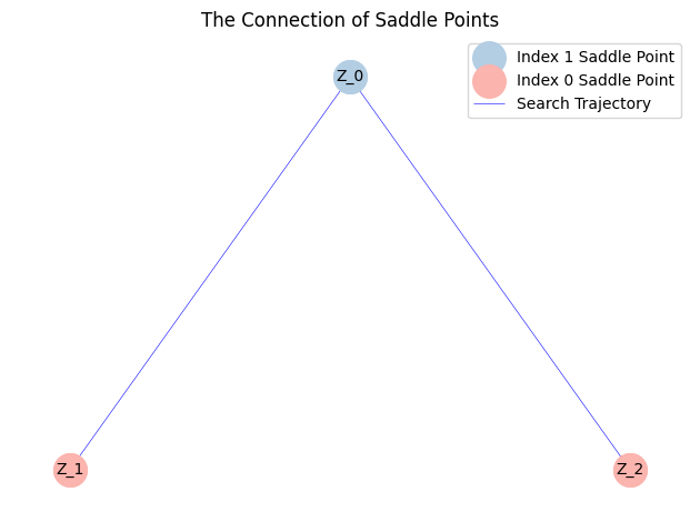
However, the Müller-Brown Potential describes a typical system with a multimodal distribution. The solution landscape shown above is therefore incomplete. Then, we restarted the search from a local minimum:

MyLandscape.RestartFromSaddle(1,-np.array([[-0.01],[0]]),1)
# Calculate

From initial point search index-1:
------------------------------


Iteration: 100|| Norm of gradient: 3.005940
Iteration: 200|| Norm of gradient: 0.692884
Iteration: 300|| Norm of gradient: 0.000017
Non-degenerate saddle point identified: Morse index =1 (number of negative eigenvalues).


From saddle point (index-1, ID-3) search index-0:
------------------------------


Iteration: 100|| Norm of gradient: 0.002417
Non-degenerate saddle point identified: Morse index =0 (number of negative eigenvalues).


From saddle point (index-1, ID-3) search index-0:
------------------------------


Iteration: 100|| Norm of gradient: 0.343433
Iteration: 200|| Norm of gradient: 0.000033
Non-degenerate saddle point identified: Morse index =0 (number of negative eigenvalues).


From saddle point (index-1, ID-3) search index-0:
------------------------------


Iteration: 100|| Norm of gradient: 0.343433
Iteration: 200|| Norm of gradient: 0.000033
Non-degenerate saddle point identified: Morse index =0 (number of negative eigenvalues).


From saddle point (index-1, ID-3) search index-0:
------------------------------


Iteration: 100|| Norm of gradient: 0.002417
Non-degenerate saddle point identified: Morse index =0 (number of negative eigenvalues).

MyLandscape.DrawTrajectory(ContourGridNum=100, ContourGridOut=25, DetailedTraj=True)
# Draw the search path. But because of the large dimension, we cannot draw the picture.

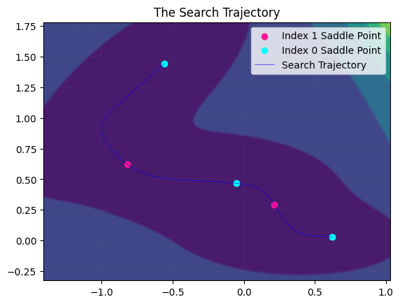
From the output, we can find a complete solution landscape.

MyLandscape.DrawConnection()
MyLandscape.Save('output/Ex_MBP','pickle')
# Save the data