High-Index Saddle Dynamics
1 What is an Index-$k$ Saddle Point($k$-saddle)
Given a twice Fréchet differentiable energy functional $E(\boldsymbol{x})$ defined on a real Hilbert space $\mathcal{H}$ with an inner product $\langle \cdot,\cdot \rangle$, we let $\boldsymbol{F}(\boldsymbol{x}) = -\nabla E(\boldsymbol{x})$ denote its natural force and $\mathbb{G}(\boldsymbol{x}) = \nabla^2E(\boldsymbol{x})$ denote its Hessian matrix.By the Riesz representation theorem, we regard $\boldsymbol{F}(\boldsymbol{x})$ as an element of $\mathcal{H}$.
-
$\boldsymbol{\hat{x}} \in \mathcal{H}$ is called a critical point of $E(\boldsymbol{x})$ if $\lVert \boldsymbol{F}(\boldsymbol{\hat{x}}) \rVert = 0$.
-
A critical point of $E(\boldsymbol{x})$ that is not a local extremum is called a saddle point of $E(\boldsymbol{x})$. Especially, sometimes we also refer to a local minimum as an index-$0$ saddle point and a local maximum as an index-$d$ saddle point (where $d$ is the system dimension).
-
A critical point $\boldsymbol{\hat{x}}$ is called nondegenerate if $\mathbb{G}(\boldsymbol{\hat{x}})$ has a bounded inverse.
-
According to Morse theory, the index (Morse index) of a nondegenerate critical point $\boldsymbol{\hat{x}}$ is the maximal dimension of a subspace $\mathcal{K}$ on which the operator $\mathbb{G}(\boldsymbol{\hat{x}})$ is negative definite. Our goal is to find an index-$k$ saddle point ,or for short,$k$-saddle,on the potential energy surface(PES).
-
For simplicity, we assume that the dimension of $\mathcal{H}$ is $d$ and write the inner product $\langle \boldsymbol{x}, \boldsymbol{y} \rangle$ as $\boldsymbol{x}^{\top} \boldsymbol{y}$.
Next, we provide an intuitive understanding of the index of a saddle point from the perspective of eigenvalues and eigenvectors, which will be useful for developing the subsequent discussion.
We note that the Hessian matrix is a real symmetric matrix (owing to the earlier assumption of quadratic Fréchet differentiability), and thus it is orthogonally similar to a diagonal matrix, meaning there exist an orthogonal matrix $\mathbb{T}$ and a diagonal matrix $\mathbb{D}$ such that $\mathbb{T}^{-1} \mathbb{G}(\boldsymbol{\hat{x}}) \mathbb{T} = \mathbb{D}$. In fact, the diagonal elements of this diagonal matrix are the eigenvalues $\hat{\lambda}_1, \hat{\lambda}_2, \ldots, \hat{\lambda}_d$ of the real symmetric matrix, and without loss of generality we can assume that $\hat{\lambda}_1 \leq \hat{\lambda}_2 \leq \ldots \leq \hat{\lambda}_d$, with the corresponding eigenvectors $\boldsymbol{\hat{v}}_1, \boldsymbol{\hat{v}}_2, \ldots, \boldsymbol{\hat{v}}_d$.
It can be proven that for a nondegenerate critical point $\hat{x}$, if \(\hat{\lambda}_1 \leq \ldots \leq \hat{\lambda}_k < 0 < \hat{\lambda}_{k+1} \leq \ldots \leq \hat{\lambda}_d\) ,then $k$ is the index of the saddle point.
On one hand, $\mathbb{G}(\boldsymbol{\hat{x}})$ is negative definite on the subspace $\hat{\mathcal{V}}$ spanned by $\boldsymbol{\hat{v}}_1, \boldsymbol{\hat{v}}_2, \ldots, \boldsymbol{\hat{v}}_k$, so $\boldsymbol{\hat{x}}$ is at least a $k$-saddle point;
On the other hand, for any subspace $\mathcal{K’}$ of $\mathcal{H}$ with dimension $k+1$ , the subspace $\hat{\mathcal{V}}^{\perp}$ spanned by \(\boldsymbol{\hat{v}}_{k+1}, \ldots, \boldsymbol{\hat{v}}_d\) intersects with $\mathcal{K’}$ non-trivially (otherwise, by adding \(\boldsymbol{\hat{v}}_{k+1}, \ldots, \boldsymbol{\hat{v}}_d\) to $\mathcal{K’}$, we would generate a space with dimension $d+1$, which is a contradiction!). Let a non-zero element in the intersection be
\[\boldsymbol{w} = \sum_{i=k+1}^{d} a_i \boldsymbol{\hat{v}}_i\]then we have
\[\boldsymbol{w}^{\top} \mathbb{G}(\hat{x}) \boldsymbol{w} = \sum_{i=k+1}^{d} a_i \boldsymbol{\hat{v}}_i^{\top} \sum_{i=k+1}^{d} \hat{\lambda}_i a_i \boldsymbol{\hat{v}}_i = \sum_{i=k+1}^{d} \hat{\lambda}_i a_i^2 > 0\]Thus, $\mathbb{G}(\boldsymbol{\hat{x}})$ is not negative definite on $\mathcal{K’}$, meaning the index of $\boldsymbol{\hat{x}}$ is $k$.
In fact, if one is familiar with the canonical form of a real symmetric matrix, it can be seen that the index of a saddle point here is essentially the negative inertia index of the Hessian matrix.
2 Transforming the Search for a $k$-saddle into an Optimization Problem
Continuing with the previous notation, note that $\mathbb{G}(\boldsymbol{\hat{x}})$ is negative definite on $\hat{\mathcal{V}}$ and positive definite on its orthogonal complement $\hat{\mathcal{V}}^{\perp}$, which implies that $\boldsymbol{\hat{x}}$ is a local maximum on the linear manifold $\boldsymbol{\hat{x}} + \hat{\mathcal{V}}$ and a local minimum on the linear manifold $\boldsymbol{\hat{x}} + \hat{\mathcal{V}}^{\perp}$.
Consider \(\boldsymbol{\hat{x}}_{\hat{\mathcal{V}}}, \boldsymbol{\hat{x}}_{\hat{\mathcal{V}}^{\perp}}\) as the projections of $\boldsymbol{\hat{x}}$ onto \(\hat{\mathcal{V}}, \hat{\mathcal{V}}^{\perp}\) , respectively, then \((\boldsymbol{v}, \boldsymbol{w}) = (\boldsymbol{\hat{x}}_{\hat{\mathcal{V}}}, \boldsymbol{\hat{x}}_{\hat{\mathcal{V}}^{\perp}})\) is a solution to the minimax problem
\[\min_{\boldsymbol{w} \in \hat{\mathcal{V}}^{\perp}} \max_{\boldsymbol{v} \in \hat{\mathcal{V}}} E(\boldsymbol{v} + \boldsymbol{w}).\]However, this is not a classical minimax problem because the space $\hat{\mathcal{V}}$ is unknown. Therefore, in the process of solving the optimization problem, our iterative method should include two parts: one is to update $\boldsymbol{v}$ and $\boldsymbol{w}$ (in this problem, also update $\boldsymbol{x} = \boldsymbol{v} + \boldsymbol{w}$), and the other is to update the space $\mathcal{V}$ (which is used to approximate $\hat{\mathcal{V}}$, typically described by the subspace spanned by the eigenvectors corresponding to the $k$ smallest eigenvalues of the Hessian matrix at the current $\boldsymbol{x}$).
3 The Dynamics of $\boldsymbol{x}$
Updating $\boldsymbol{x}$ intuitively involves making the projection of $\boldsymbol{\dot{x}}$ onto the space $\mathcal{V}$, \(\mathcal{P}_{\mathcal{V}} \boldsymbol{\dot{x}}\) , the ascent direction of the energy function \(E(\boldsymbol{x})\) , while the projection onto its complement \(\mathcal{V}^{\perp}\) , \(\mathcal{P}_{\mathcal{V}^{\perp}} \boldsymbol{\dot{x}}\) , is the descent direction.
In particular, since the natural force $\boldsymbol{F}(\boldsymbol{x}) = -\nabla E(\boldsymbol{x})$ is the steepest descent direction, we can consider setting \(\mathcal{P}_{\mathcal{V}} \boldsymbol{\dot{x}} = -\mathcal{P}_{\mathcal{V}} \boldsymbol{F}(\boldsymbol{x})\) and \(\mathcal{P}_{\mathcal{V}^{\perp}} \boldsymbol{\dot{x}} = \mathcal{P}_{\mathcal{V}^{\perp}} \boldsymbol{F}(\boldsymbol{x}) = \boldsymbol{F}(\boldsymbol{x}) - \mathcal{P}_{\mathcal{V}} \boldsymbol{F}(\boldsymbol{x})\) , and then introducing two positive relaxation constants $\beta_{\mathcal{V}}$ and $\beta_{\mathcal{V}^{\perp}}$, we can give the dynamics of $\boldsymbol{x}$ as
\[\boldsymbol{\dot{x}} = \beta_{\mathcal{V}} (-\mathcal{P}_{\mathcal{V}} \boldsymbol{F}(\boldsymbol{x})) + \beta_{\mathcal{V}^{\perp}} (\boldsymbol{F}(\boldsymbol{x}) - \mathcal{P}_{\mathcal{V}} \boldsymbol{F}(\boldsymbol{x})).\]Furthermore, if we simply set $\beta_{\mathcal{V}} = \beta_{\mathcal{V}^{\perp}} = \beta$, the equation becomes
\[\beta^{-1} \boldsymbol{\dot{x}} = \boldsymbol{F}(\boldsymbol{x}) - 2 \mathcal{P}_{\mathcal{V}} \boldsymbol{F}(\boldsymbol{x}) \tag{1}\]In particular, if a set of standard orthonormal basis $\boldsymbol{v_1}, \boldsymbol{v_2}, \ldots, \boldsymbol{v_k}$ for the space $\mathcal{V}$ is given, the projection transformation is \(\mathcal{P}_{\mathcal{V}} = \sum_{i=1}^{k} \boldsymbol{v}_i \boldsymbol{v}^{\top}_i\) , so equation (1) becomes
\[\beta^{-1} \boldsymbol{\dot{x}} = \left(\mathbb{I} - 2 \sum_{i=1}^{k} \boldsymbol{v}_i \boldsymbol{v}^{\top}_i \right) \boldsymbol{F}(\boldsymbol{x}) \tag{2}\]where $\mathbb{I}$ is the identity matrix.
4 Updating the Subspace $\mathcal{V}$
Our goal is to use $\mathcal{V}$ to approximate $\hat{\mathcal{V}}$. Note that $\hat{\mathcal{V}}$ is the subspace spanned by the eigenvectors corresponding to the $k$ smallest eigenvalues of the Hessian matrix $\mathbb{G}(\boldsymbol{\hat{x}})$, so we can consider using the subspace generated by the eigenvectors corresponding to the $k$ smallest eigenvalues of $\mathbb{G}(\boldsymbol{x})$ as $\mathcal{V}$.
4.1 Basic Method: Transforming to a Constrained Optimization Problem and Constructing Dynamics Using the Gradient Flow of the Lagrangian Function
Let’s first focus on the simplest case: how to find the smallest eigenvalue and its corresponding eigenvector? We can solve the constrained optimization problem
\[\min_{\boldsymbol{v}_1} \langle \boldsymbol{v}_1, \mathbb{G}(\boldsymbol{x}) \boldsymbol{v}_1 \rangle \quad \text{s.t.} \quad \langle \boldsymbol{v}_1, \boldsymbol{v}_1 \rangle = 1\]to achieve it.
Similarly, given $\boldsymbol{v}1, \boldsymbol{v}_2, \ldots, \boldsymbol{v}{i-1}$, to find the $i$-th smallest eigenvalue and its corresponding eigenvector, we can solve the following constrained optimization problem:
\[\min_{\boldsymbol{v}_i} \langle \boldsymbol{v}_i, \mathbb{G}(\boldsymbol{x}) \boldsymbol{v}_i \rangle \quad \text{s.t.} \quad \langle \boldsymbol{v}_i, \boldsymbol{v}_j \rangle = \delta_{ij} \quad j=1,2,\ldots,i \tag{3}\]where
\[\delta_{ij} = \begin{cases} 1 & \text{if } i = j \\ 0 & \text{if } i \neq j \end{cases}\]We consider the dynamics of this series of constrained optimization problems. Consider the Lagrangian function
\[\mathcal{L}_i(\boldsymbol{v}_i; \xi^{(i)}_1, \ldots, \xi^{(i)}_{i-1}, \xi^{(i)}_i) = \langle \boldsymbol{v}_i, \mathbb{G}(\boldsymbol{x}) \boldsymbol{v}_i \rangle - \xi^{(i)}_i (\langle \boldsymbol{v}_i, \boldsymbol{v}_i \rangle - 1) - \sum_{j=1}^{i-1} \xi^{(i)}_j \tag{4}\]Taking the gradient with respect to $\boldsymbol{v}_i$, we get
\[\frac{\partial}{\partial \boldsymbol{v}_i} \mathcal{L}_i(\boldsymbol{v}_i; \xi^{(i)}_1, \ldots, \xi^{(i)}_{i-1}, \xi^{(i)}_i) = 2 \mathbb{G}(\boldsymbol{x}) \boldsymbol{v}_i - 2 \xi^{(i)}_i \boldsymbol{v}_i - \sum_{j=1}^{i-1} \xi^{(i)}_j \boldsymbol{v}_j\]Now, taking a relaxation constant $\gamma > 0$, the dynamics of $\boldsymbol{v}_i$ given by the gradient flow of the Lagrangian function (with undetermined coefficients) is
\[\begin{aligned} \boldsymbol{\dot{v}}_i &= -\frac{\gamma}{2} \frac{\partial}{\partial \boldsymbol{v}_i} \mathcal{L}_i(\boldsymbol{v}_i; \xi^{(i)}_1, \ldots, \xi^{(i)}_{i-1}, \xi^{(i)}_i) \nonumber \\ &= -\gamma \left( \mathbb{G}(\boldsymbol{x}) \boldsymbol{v}_i - \xi^{(i)}_i \boldsymbol{v}_i - \frac{1}{2} \sum_{j=1}^{i-1} \xi^{(i)}_j \boldsymbol{v}_j \right) \label{the dynamics of v_i with undetermined coefficient}\end{aligned}\]The factor $-\frac{\gamma}{2}$ is used here instead of $-\gamma$ for simplicity in the expression later. The next step is to determine each $\xi_i$. Notice the equality constraints
\[c^{(i)}_i(t) = \langle \boldsymbol{v}_i, \boldsymbol{v}_i \rangle - 1 = 0\] \[c^{(i)}_j(t) = \langle \boldsymbol{v}_i, \boldsymbol{v}_j \rangle = 0 \quad j=1,2,\ldots,i-1\]To ensure that the initial values satisfy the equality constraints, we require:
\[\dot{c}^{(i)}_i(t) = 2 \langle \boldsymbol{\dot{v}}_i, \boldsymbol{v}_i \rangle = 0\] \[\dot{c}^{(i)}_j(t) = \langle \boldsymbol{\dot{v}}_i, \boldsymbol{v}_j \rangle + \langle \boldsymbol{v}_i, \boldsymbol{\dot{v}}_j \rangle = 0 \quad j=1,2,\ldots,i-1\]Substituting equation (4) into these equations (solving in the order of superscripts), we obtain
\[\xi^{(i)}_i = \langle \boldsymbol{v}_i, \mathbb{G} \boldsymbol{v}_i \rangle\] \[\xi^{(i)}_j = 4 \langle \boldsymbol{v}_j, \mathbb{G} \boldsymbol{v}_i \rangle \quad j=1,2,\ldots,i-1\]Substituting these back into equation (4), we obtain the final dynamics of $\boldsymbol{v}_i$:
\[\begin{aligned} \gamma^{-1} \boldsymbol{\dot{v}}_i &= - \mathbb{G}(\boldsymbol{x}) \boldsymbol{v}_i + \langle \boldsymbol{v}_i, \mathbb{G} \boldsymbol{v}_i \rangle \boldsymbol{v}_i + 2 \sum_{j=1}^{i-1} \langle \boldsymbol{v}_j, \mathbb{G} \boldsymbol{v}_i \rangle \boldsymbol{v}_j \nonumber \\ &= - (\mathbb{I} - \boldsymbol{v}_i \boldsymbol{v}_i^\top - 2 \sum_{j=1}^{i-1} \boldsymbol{v}_j \boldsymbol{v}_j^\top) \mathbb{G}(\boldsymbol{x}) \boldsymbol{v}_i \quad i=1,2,\ldots,k \end{aligned} \tag{5}\]Combining equations (2) and (5), we obtain the dynamics of the entire problem:
\[\begin{cases} & \beta^{-1} \boldsymbol{\dot{x}} = \left( \mathbb{I} - 2 \sum_{i=1}^{k} \boldsymbol{v}_i \boldsymbol{v}_i^\top \right) \boldsymbol{F}(\boldsymbol{x}) \\ & \gamma^{-1} \boldsymbol{\dot{v}}_i = - \left( \mathbb{I} - \boldsymbol{v}_i \boldsymbol{v}_i^\top - 2 \sum_{j=1}^{i-1} \boldsymbol{v}_j \boldsymbol{v}_j^\top \right) \mathbb{G}(\boldsymbol{x}) \boldsymbol{v}_i \quad i=1,2,\ldots,k \end{cases} \tag{6}\]4.2 Cases Requiring Numerical Approximation of the Hessian Matrix — Shrinking Dimer Method
In equation (6), if the exact Hessian is available, then it can be used directly. However, for many problems, the Hessian matrix cannot be computed or the cost of computation is too high. We need numerical approximation methods to handle the Hessian matrix. In particular, in equation (6), we don’t need to approximate the entire matrix, but only need to handle the form of the Hessian matrix multiplied by a vector $\mathbb{G}(\boldsymbol{x}) \boldsymbol{v}_i$, which can be done through finite differences.
Consider approximating the vector $\mathbb{G}(\boldsymbol{x}) \boldsymbol{v}$, noting that
\[-\boldsymbol{F}(\boldsymbol{x}+l\boldsymbol{v}) \approx \nabla E(\boldsymbol{x}+l\boldsymbol{v}) = \nabla E(\boldsymbol{x}) + \mathbb{G}(\boldsymbol{x}) l \boldsymbol{v} + \mathcal{O}(\lVert l \boldsymbol{v} \rVert^2) \quad (l \to 0)\] \[-\boldsymbol{F}(\boldsymbol{x}-l\boldsymbol{v}) \approx \nabla E(\boldsymbol{x}-l\boldsymbol{v}) = \nabla E(\boldsymbol{x}) - \mathbb{G}(\boldsymbol{x}) l \boldsymbol{v} + \mathcal{O}(\lVert l \boldsymbol{v} \rVert^2) \quad (l \to 0)\]Thus, we can approximate
\[\boldsymbol{H}(\boldsymbol{x}, \boldsymbol{v}, l) = -\frac{\boldsymbol{F}(\boldsymbol{x}+l\boldsymbol{v}) - \boldsymbol{F}(\boldsymbol{x}-l\boldsymbol{v})}{2l} \approx \mathbb{G}(\boldsymbol{x}) \boldsymbol{v} \tag{7}\]In fact, the dimer method intuitively estimates the Hessian matrix at the center point $\boldsymbol{x}$ by using the gradients at the points $\boldsymbol{x}+l\boldsymbol{v}$ and $\boldsymbol{x}-l\boldsymbol{v}$. The shrinking dimer refers to the process of bringing these two points closer together until they eventually converge at the center. This estimation is exact in the limit, but in numerical calculations, $l$ should not become too small due to the appearance of $l$ in the denominator to ensure numerical stability.
The "shrinking" process in numerical algorithms can be implemented by introducing dynamics for $l$. The simplest choice is to consider $\dot{l} = -l$, corresponding to the exponential decay of the dimer length. This gives the dynamics for the entire problem when the Hessian matrix needs to be numerically approximated:
\[\begin{cases} & \beta^{-1} \boldsymbol{\dot{x}} = \left( \mathbb{I} - 2 \sum_{i=1}^{k} \boldsymbol{v}_i \boldsymbol{v}_i^\top \right) \boldsymbol{F}(\boldsymbol{x}) \\ & \gamma^{-1} \boldsymbol{\dot{v}}_i = - \left( \mathbb{I} - \boldsymbol{v}_i \boldsymbol{v}_i^\top - 2 \sum_{j=1}^{i-1} \boldsymbol{v}_j \boldsymbol{v}_j^\top \right) \boldsymbol{H}(\boldsymbol{x}, \boldsymbol{v}, l) \quad i=1,2,\ldots,k \\ & \dot{l} = -l \end{cases}\]The linear stability of this method can be found in Reference [1].
5 Direct Discretization of HiSD Dynamics
We directly discretize the dynamics given above and present the following algorithm:
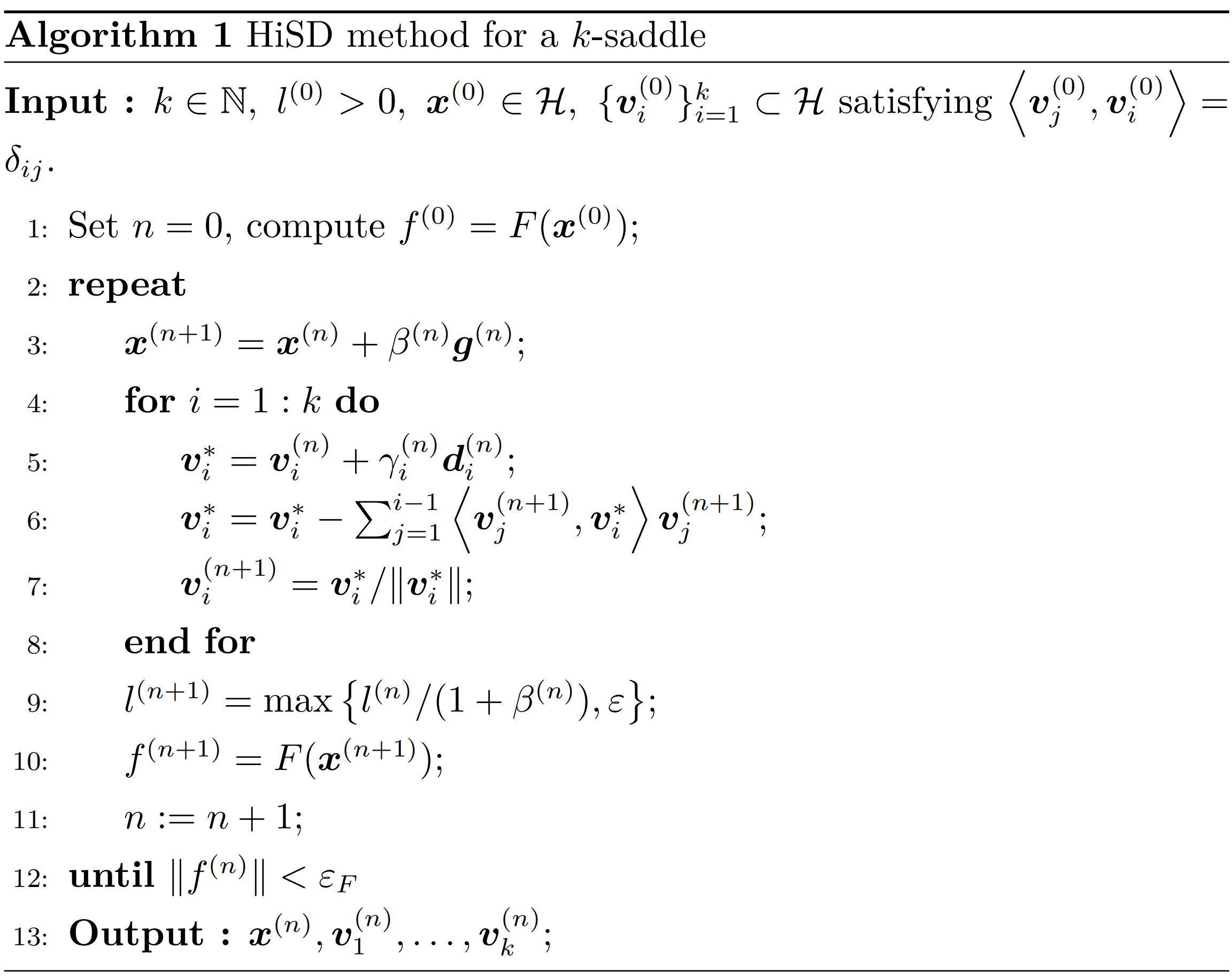
where
\[\boldsymbol{g}^{(n)} = \boldsymbol{f}^{(n)} - 2 \sum_{i=1}^k \left\langle \boldsymbol{v}_i^{(n)}, \boldsymbol{f}^{(n)} \right\rangle \boldsymbol{v}_i^{(n)}\] \[\boldsymbol{d}_i^{(n)} = -\boldsymbol{u}_i^{(n)} + \left\langle \boldsymbol{v}_i^{(n)}, \boldsymbol{u}_i^{(n)} \right\rangle \boldsymbol{v}_i^{(n)} + \sum_{j=1}^{i-1} 2 \left\langle \boldsymbol{v}_j^{(n)}, \boldsymbol{u}_i^{(n)} \right\rangle \boldsymbol{v}_j^{(n)}\] \[\boldsymbol{u}_i^{(n)} = H\left( \boldsymbol{x}^{(n+1)}, \boldsymbol{v}_i^{(n)}, l^{(n)} \right)\]Step 6 and 7 use Gram-Schmidt orthogonalization to maintain the orthogonality condition. Step 9 introduces $\varepsilon$ to prevent $l^{(n)}$ in the denominator of $H\left( \boldsymbol{x}^{(n+1)}, \boldsymbol{v}_i^{(n)}, l^{(n)} \right)$ from becoming too small, ensuring numerical stability.
Note that the dynamics provided earlier essentially give the iteration direction in the discretized iteration process, while the algorithm above also involves quantities like $\beta^{(n)}$ and $\gamma_i^{(n)}$, which are step sizes in the iterative algorithm. Various methods for selecting these step sizes are introduced in the next section.
6 Selection of Iterative Step Sizes
In simple terms, typical methods for selecting step sizes are as follows:
6.1 Explicit Euler Method
Set $\beta^{(n)} = \gamma_i^{(n)} = \Delta t > 0$ as a fixed constant, where $\Delta t$ should not be too small, as it may result in slow convergence, nor should it be too large, as it may cause the algorithm to diverge.
6.2 Line Search Method (for $\beta^{(n)}$)
Minimize $|\boldsymbol{F}(\boldsymbol{x}^{(n)} + \beta^{(n)} \boldsymbol{g}^{(n)})|^2$ with respect to $\beta^{(n)}$, either using exact or inexact line search. A practical approach is to set an upper bound $\tau$ for $\beta^{(n)} |\boldsymbol{g}^{(n)}|$ to avoid large jumps between states; simultaneously, set a lower bound for $\beta^{(n)}$ so that it can escape from the neighborhood of a critical point, which is different from finding the minimizer.
6.3 BB Gradient Method
Let $\Delta \boldsymbol{x}^{(n)} = \boldsymbol{x}^{(n)} - \boldsymbol{x}^{(n-1)}$ and $\Delta \boldsymbol{g}^{(n)} = \boldsymbol{g}^{(n)} - \boldsymbol{g}^{(n-1)}$. Based on the quasi-Newton method, we solve the optimization problems
\[\min_{\beta^{(n)}} \|\Delta \boldsymbol{x}^{(n)} / \beta^{(n)} - \boldsymbol{g}^{(n)}\|\] \[\min_{\beta^{(n)}} \|\Delta \boldsymbol{x}^{(n)} - \beta^{(n)} \boldsymbol{g}^{(n)}\|\]to obtain the BB1 and BB2 step sizes:
\[\beta_{\text{BB1}}^{(n)} = \frac{\langle \Delta \boldsymbol{x}^{(n)}, \Delta \boldsymbol{x}^{(n)} \rangle}{\langle \Delta \boldsymbol{x}^{(n)}, \Delta \boldsymbol{g}^{(n)} \rangle}\] \[\beta_{\text{BB2}}^{(n)} = \frac{\langle \Delta \boldsymbol{x}^{(n)}, \Delta \boldsymbol{g}^{(n)} \rangle}{\langle \Delta \boldsymbol{g}^{(n)}, \Delta \boldsymbol{g}^{(n)} \rangle}\]In this problem, since the denominator of the BB1 step size may become too small and cause numerical instability, we generally use the BB2 step size. Of course, similar to the line search, we can set an upper bound for $\beta^{(n)} |\boldsymbol{g}^{(n)}|$ and take the absolute value of $\beta_{\text{BB2}}^{(n)}$ to avoid negative step sizes. Combining these gives:
\[\beta^{(n)} = \min \left\{ \frac{\tau}{\|\boldsymbol{g}^{(n)}\|}, \left| \frac{\langle \Delta \boldsymbol{x}^{(n)}, \Delta \boldsymbol{g}^{(n)} \rangle}{\langle \Delta \boldsymbol{g}^{(n)}, \Delta \boldsymbol{g}^{(n)} \rangle} \right| \right\}\]For $\gamma_i^{(n)}$, using the BB2 step size gives
\[\gamma_i^{(n)} = \left| \frac{\langle \Delta \boldsymbol{v}_i^{(n)}, \Delta \boldsymbol{d}_i^{(n)} \rangle}{\langle \Delta \boldsymbol{d}_i^{(n)}, \Delta \boldsymbol{d}_i^{(n)} \rangle} \right|\]7 An Alternative Update of $\mathcal{V}$ — Application of LOBPCG Method
In fact, besides directly discretizing the dynamics of HiSD, we can also consider combining other classical methods with the dimer method to update $\mathcal{V}$. Essentially, this still involves solving the problem of finding the eigenvectors corresponding to the $k$ smallest eigenvalues. Here, we use the LOBPCG (Locally Optimal Block Preconditioned Conjugate Gradient) method, as it balances both efficiency and speed well.
7.1 Basic Idea of the Method
The Rayleigh quotient optimization problem (3) over the entire space is transformed into an approximate solution in a subspace $\mathcal{U}$, and with multiple iterations, the information in this subspace gradually improves, leading to better approximations. That is, the eigenvectors found are closer to the $k$ smallest eigenvectors in the full space. By transforming it into a subspace eigenvalue problem, we can solve for the eigenvalues of a smaller matrix.
Specifically, the problem we face is:
\[\min \sum_{i=1}^{k} \langle \boldsymbol{v}_i, \mathbb{G}(\boldsymbol{x}) \boldsymbol{v}_i \rangle \quad \text{s.t.} \quad \boldsymbol{v}_i \in \mathcal{U}, \langle \boldsymbol{v}_i, \boldsymbol{v}_j \rangle = \delta_{ij}\]In the actual algorithm, we can consider performing one LOBPCG iteration after each $\boldsymbol{x}$ update, or we can choose to perform multiple iterations. Below is the case with just one iteration, where the superscript $(n)$ denotes the number of $\boldsymbol{x}$ updates, and particularly, in this case, also the number of $\boldsymbol{v}_i$ updates.
In the LOBPCG method, we apply the symmetric positive-definite preconditioner $\mathbb{T}$ to the residual vector to obtain
\[\boldsymbol{w}_i^{(n)} = \mathbb{T} \left( \mathbb{G}(\boldsymbol{x}^{(n+1)}) \boldsymbol{v}_i^{(n)} - \left\langle \boldsymbol{v}_i^{(n)}, \mathbb{G}(\boldsymbol{x}^{(n+1)}) \boldsymbol{v}_i^{(n)} \right\rangle \boldsymbol{v}_i^{(n)} \right)\]Then, we combine the current and previous approximate eigenvectors to form the subspace in the LOBPCG method:
\[\mathcal{U}_{\text{CG}}^{(n)} = \text{span} \left\{ \boldsymbol{v}_i^{(n-1)}, \boldsymbol{v}_i^{(n)}, \boldsymbol{w}_i^{(n)}, i=1,2,\ldots,k \right\}\]Let $\boldsymbol{w}_{i+k}^{(n)} = \boldsymbol{v}_i^{(n-1)}, i = 1, 2, \ldots, k$, and perform Gram-Schmidt orthogonalization:
\[\tilde{\boldsymbol{w}}_i^{(n)} = \boldsymbol{w}_i^{(n)} - \sum_{j=1}^{k} \left\langle \boldsymbol{w}_i^{(n)}, \boldsymbol{v}_j^{(n)} \right\rangle \boldsymbol{v}_j^{(n)} - \sum_{\substack{j=1 \\ \|\tilde{\boldsymbol{w}}_j^{(n)}\| > \epsilon_w}}^{i-1} \frac{\left\langle \boldsymbol{w}_i^{(n)}, \tilde{\boldsymbol{w}}_j^{(n)} \right\rangle}{\left\| \tilde{\boldsymbol{w}}_j^{(n)} \right\|^2} \tilde{\boldsymbol{w}}_j^{(n)}, i=1,2,\ldots, 2k\]Vectors with small norms are discarded to maintain numerical stability. This results in an orthogonal matrix of column vectors of size $n \times K$ (where $k \leq K \leq 3k$):
\[\mathbb{U}_{\text{CG}}^{(n)} = \left[ \boldsymbol{v}_1^{(n)}, \ldots, \boldsymbol{v}_k^{(n)}, \frac{\tilde{\boldsymbol{w}}_i^{(n)}}{\|\tilde{\boldsymbol{w}}_i^{(n)}\|} : \|\tilde{\boldsymbol{w}}_i^{(n)}\| > \epsilon_w, i = 1, \ldots, 2k \right] \tag{8}\]Thus, the vectors in the subspace can be approximated as $\mathbb{U}_{\text{CG}}^{(n)} \boldsymbol{\eta}$, where $\boldsymbol{\eta} \in \mathbb{R}^{K \times 1}$.
Next, finding the $k$ smallest eigenvalues and corresponding eigenvectors in $\mathcal{U}_{\text{CG}}^{(n)}$ is equivalent to solving for $\boldsymbol{\eta}$ such that
\[\mathbb{G}(\boldsymbol{x}^{(n+1)}) \mathbb{U}_{\text{CG}}^{(n)} \boldsymbol{\eta} = \lambda \mathbb{U}_{\text{CG}}^{(n)} \boldsymbol{\eta}\]That is,
\[(\mathbb{U}_{\text{CG}}^{(n)})^{\top} \mathbb{G}(\boldsymbol{x}^{(n+1)}) \mathbb{U}_{\text{CG}}^{(n)} \boldsymbol{\eta} = \lambda \boldsymbol{\eta} \tag{9}\]Thus, we only need to solve for the $k$ smallest eigenvalues and corresponding eigenvectors of the $K \times K$ symmetric matrix \((\mathbb{U}_{\text{CG}}^{(n)})^{\top} \mathbb{G}(\boldsymbol{x}^{(n+1)}) \mathbb{U}_{\text{CG}}^{(n)}\) , and once they are found, we can recover the eigenvectors in the original space by multiplying the eigenvectors by $\mathbb{U}_{\text{CG}}^{(n)}$.
There are various methods to solve for the eigenvalues of a small symmetric matrix (generally $K$ is small), such as the QR method, Jacobi method, etc.
In fact, the matrix $\mathbb{G}(\boldsymbol{x}^{(n+1)})$ can still be handled using the dimer method, as $\mathbb{G}(\boldsymbol{x}^{(n+1)}) \mathbb{U}_{\text{CG}}^{(n)}$ essentially still involves the structure where we only need to focus on multiplying the Hessian matrix by a vector, which we already approximated earlier:
\[\mathbb{G}(\boldsymbol{x}^{(n+1)}) \boldsymbol{v}_i^{(n)} \approx \boldsymbol{u}_i^{(n)} = H \left( \boldsymbol{x}^{(n+1)}, \boldsymbol{v}_i^{(n)}, l^{(n)} \right)\]Similarly, we define
\[\boldsymbol{y}_i^{(n)} = \boldsymbol{H} \left( \boldsymbol{x}^{(n+1)}, \frac{\tilde{\boldsymbol{w}}_i^{(n)}}{\|\tilde{\boldsymbol{w}}_i^{(n)}\|}, l^{(n)} \right)\]Using the formula (7), we can approximate
\[\mathbb{Y}_{\text{CG}}^{(n)} = \left[ \boldsymbol{u}_1^{(n)}, \ldots, \boldsymbol{u}_k^{(n)}, \boldsymbol{y}_i^{(n)} : \|\tilde{\boldsymbol{w}}_i^{(n)}\| > \epsilon_w, i = 1, \ldots, 2k \right] \tag{10}\]to approximate $\mathbb{G}(\boldsymbol{x}^{(n+1)}) \mathbb{U}_{\text{CG}}^{(n)}$. Thus, we can use
\[\mathbb{P}_{\text{CG}}^{(n)} = (\mathbb{U}_{\text{CG}}^{(n)})^{\top} \mathbb{Y}_{\text{CG}}^{(n)}\]to approximate \((\mathbb{U}_{\text{CG}}^{(n)})^{\top} \mathbb{G}(\boldsymbol{x}^{(n+1)}) \mathbb{U}_{\text{CG}}^{(n)}\) in equation (9). To maintain the symmetry of \(\mathbb{P}_{\text{CG}}^{(n)}\) due to numerical errors, it is better to use \((\mathbb{P}_{\text{CG}}^{(n)} + (\mathbb{P}_{\text{CG}}^{(n)})^{\top}) / 2\) as a substitute for $\mathbb{P}_{\text{CG}}^{(n)}$.
Algorithm Framework
Summarizing the content of the previous subsection, we obtain the general framework of the HiSD-LOBPCG algorithm:
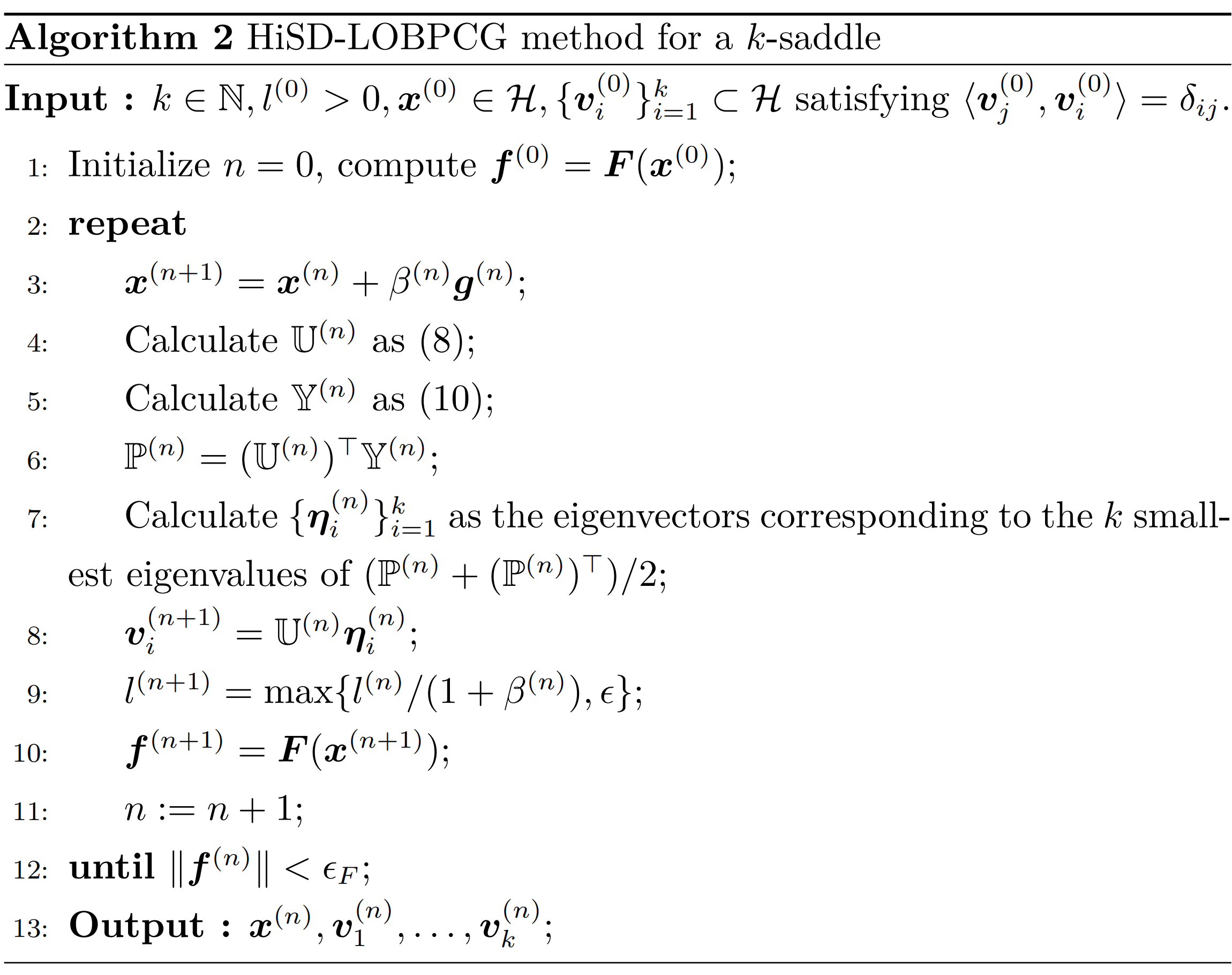
Note that the step size selection only appears in the choice of $\beta^{(n)}$ in line 3, which can be referred to in Section 6.
8 Summary
Previously, we introduced the background of the problems targeted by the HiSD series of algorithms and explained the significance of solving for $k$-saddle. In this chapter, we first described $k$-saddle in more detail from the perspective of eigenvalues. Subsequently, we transformed the problem of solving for $k$-saddle into an optimization problem and provided the dynamics for this problem. Direct discretization of these dynamics led to the HiSD algorithm. Finally, based on this framework, we presented several step size selection methods to further solidify the algorithm’s implementation, as well as integrated LOBPCG into the HiSD method to offer alternative approaches to solving the problem.
9 References
- Yin, J., Zhang, L., & Zhang, P. (2019). High-index optimization-based shrinking dimer method for finding high-index saddle points. SIAM Journal on Scientific Computing, 41(6), A3576-A3595. https://doi.org/10.1137/19M1253356