Background Introduction:Construction of Solution Landscapes for Complex Systems

Many practical problems in physics, chemistry, and other fields can be reduced to the problem of finding the minima of nonlinear functions or functionals with multiple variables. These applications span materials science, soft matter, condensed matter physics, life sciences, data science, and more. A common feature of these multi-solution problems is that the energy landscape corresponding to the function or functional of the physical variables has many minima, each corresponding to a metastable state in physics, with different minima separated by energy barriers. These variables could represent the positions of amino acids in protein folding, the atomic positions in atomic clusters, continuous field variables describing the self-assembly of block copolymers, or the parameters of neural networks, among others.

The equilibrium states of nonlinear problems correspond to the stationary points (equilibrium points) that satisfy the equation $\nabla E(\boldsymbol{x})=0$. Non-degenerate stationary points on the energy landscape (i.e., points where the Hessian matrix has no zero eigenvalues) can be classified using the Morse index from Morse theory. The Morse index is the dimension of the largest negative definite subspace of the Hessian matrix at the stationary point, which is equivalent to the number of negative eigenvalues of the Hessian matrix. Specifically, a stationary point with a Morse index of 0 corresponds to a stable minimum, while an unstable saddle point has a non-zero Morse index. For example, an index-$k$ saddle point is a stationary point where the Hessian matrix has $k$ negative eigenvalues.

In particular, index-1 saddle points are often referred to as transition states, which are points located on the smallest energy barrier between two minima. The minimum energy path is a continuous curve on the energy landscape connecting two minima via the transition state. Transition states play a crucial role in many scientific fields, such as identifying critical nuclei and transition paths in phase transitions, calculating transition rates in chemical reactions, and applications in biology.

Finding all stationary points is essential for understanding the energy landscape. However, due to the instability of saddle points, computing unstable saddle points is typically much more challenging than computing stable minima. In recent years, many renowned mathematicians, physicists, and chemists have developed a series of numerical algorithms for computing rare events and index-1 saddle points. These algorithms can be broadly divided into two categories (as shown in Figure 1):

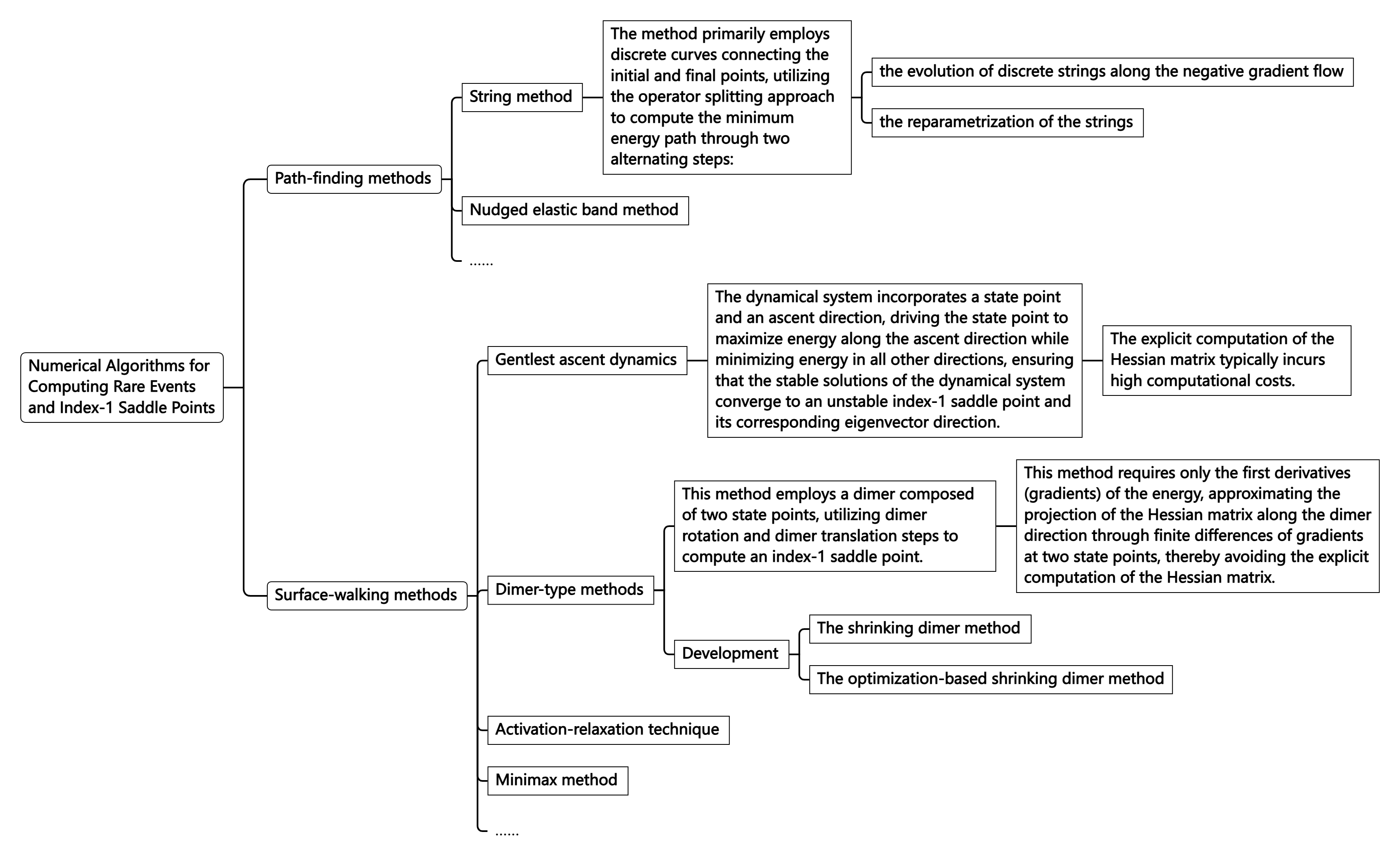Figure 1:Numerical Algorithms for Computing Rare Events and Index-1 Saddle Points

Compared to index-1 saddle points, the development of computational methods for higher-index saddle points has been much slower. This is partly because higher-index saddle points have more unstable directions, rendering some techniques used for index-1 saddle point algorithms inapplicable. Additionally, the physical significance and role of higher-index saddle points in practical problems are not yet well understood, providing insufficient motivation to address this issue. In fact, many studies have pointed out that the number of higher-index saddle points in nonlinear problems far exceeds that of minima and index-1 saddle points. Therefore, finding all solutions of complex systems and understanding the connections between different solutions remains a very important and challenging scientific problem in computational mathematics.

In recent years, we have proposed a new concept called the "solution landscape". First, we define the solution landscape as a path diagram that includes all solutions and the connections between them. Here, the solutions encompass all stable minima and unstable saddle points, while the path diagram describes the hierarchical structure where different minima are connected by corresponding index-1 saddle points, and lower-index saddle points are connected by higher-index saddle points, as shown in Figure 2{reference-type=”ref” reference=”fig:enter-label”}. We can intuitively liken the solution landscape to a family tree, where the first generation corresponds to the highest-index saddle points of the system, and the youngest generation represents the minima of the system. In this family tree, all minima are not isolated; starting from the first generation, one can follow a path to connect to every minimum.

Figure 2:Illustration of the solution landscape, where $k$-saddle represents an index-$k$ saddle point

Although the definition of the solution landscape is intuitive, numerically computing the solution landscape remains highly challenging. The main difficulty in constructing the solution landscape lies in efficiently computing the various saddle points within it. Existing methods for solving the nonlinear equation $\nabla E(\boldsymbol{x})=0$, including homotopy methods and deflation techniques, can find multiple equilibrium solutions. However, as more solutions are found, the computation of the remaining equilibrium solutions requires increasingly fine-tuning of initial guesses, making the process more difficult and hard to determine whether all solutions have been found. Moreover, these methods typically yield a collection of equilibrium solutions without revealing the connections between different solutions. To overcome this challenge, we have developed a new saddle point dynamics approach, which transforms the computation of unstable higher-index saddle points into finding stable solutions of higher-index saddle point dynamics. This approach also provides the connections between different saddle points and minima in the solution landscape.

References

1. Zhang, L. (2023). Construction of solution landscapes for complex systems. Mathematica Numerica Sinica, ​45(3), 267-283. https://doi.org/10.12286/jssx.j2023-1121